R语言实战:方差分析
本文内容来自《R 语言实战》(R in Action, 2nd),有部分修改
术语速成
组件因子
因变量 vs 自变量
均衡设计 vs 非均衡设计
单因素方差分析 one-way ANOVA,单因素组间方差分析
组内因子
单因素组内方差分析,重复测量方差分析
主效应 vs 交互效应
因素方差分析设计
混合模型方差分析
混淆因素 confounding factor
干扰变数 nuisance variable
协变量
协方差分析 ANCOVA
多元方差分析 MANOVA
多元协方差分析 MANCOVA
ANOVA 模型拟合
广义线性模型的特例
aov() 函数
定量变量
组别因子
标识变量
表达式中各项的顺序
类型1:序贯型(默认)
类型2:分层型
类型3:边界型
car 包的 Anova() 函数
单因素方差分析
library(multcomp)
head(cholesterol)
    trt response
1 1time   3.8612
2 1time  10.3868
3 1time   5.9059
4 1time   3.0609
5 1time   7.7204
6 1time   2.7139
attach(cholesterol)
table(trt)
trt
 1time 2times 4times  drugD  drugE
    10     10     10     10     10
aggregate(
  response,
  by=list(trt),
  FUN=mean
)
Group.1 x
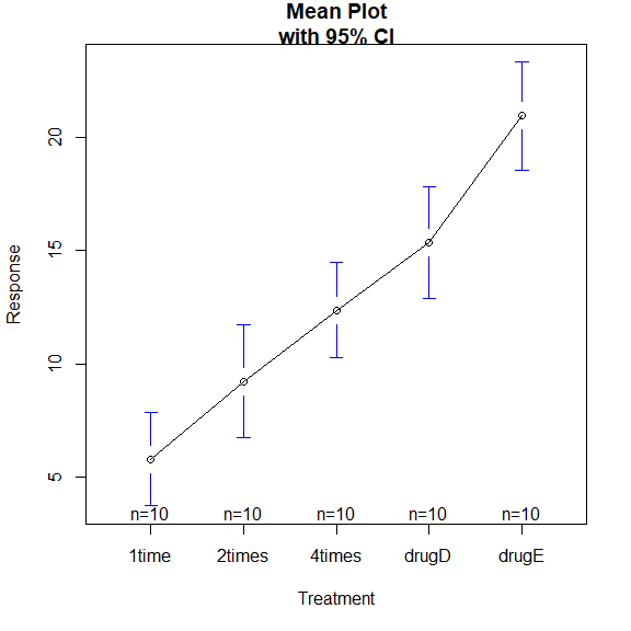
1 1time 5.78197
2 2times 9.22497
3 4times 12.37478
4 drugD 15.36117
5 drugE 20.94752
aggregate(
  response,
  by=list(trt),
  FUN=sd
)
  Group.1        x
1   1time 2.878113
2  2times 3.483054
3  4times 2.923119
4   drugD 3.454636
5   drugE 3.345003
fit <- aov(
  response ~ trt
)
summary(fit)
            Df Sum Sq Mean Sq F value   Pr(>F)
trt          4 1351.4   337.8   32.43 9.82e-13 ***
Residuals   45  468.8    10.4
---
Signif. codes:  0 ‘***’ 0.001 ‘**’ 0.01 ‘*’ 0.05 ‘.’ 0.1 ‘ ’ 1
library(gplots)
绘制各组均值及置信区间
plotmeans(
  response ~ trt,
  xlab="Treatment",
  ylab="Response",
  main="Mean Plot\nwith 95% CI"
)
detach(cholesterol)
多重比较
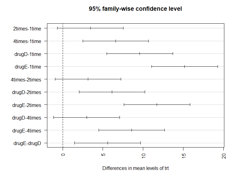
TukeyHSD() 函数,成对检验
TukeyHSD(fit)
  Tukey multiple comparisons of means
    95% family-wise confidence level

Fit: aov(formula = response ~ trt)

$trt
                  diff        lwr       upr     p adj
2times-1time   3.44300 -0.6582817  7.544282 0.1380949
4times-1time   6.59281  2.4915283 10.694092 0.0003542
drugD-1time    9.57920  5.4779183 13.680482 0.0000003
drugE-1time   15.16555 11.0642683 19.266832 0.0000000
4times-2times  3.14981 -0.9514717  7.251092 0.2050382
drugD-2times   6.13620  2.0349183 10.237482 0.0009611
drugE-2times  11.72255  7.6212683 15.823832 0.0000000
drugD-4times   2.98639 -1.1148917  7.087672 0.2512446
drugE-4times   8.57274  4.4714583 12.674022 0.0000037
drugE-drugD    5.58635  1.4850683  9.687632 0.0030633
par(las=2)
par(mar=c(5, 8, 4, 2))
plot(TukeyHSD(fit))
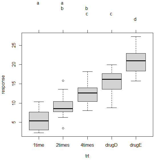
multcomp 包中的 glht() 函数
tuk <- glht(
  fit,
  linfct=mcp(trt="Tukey")
)
summary(tuk)
	 Simultaneous Tests for General Linear Hypotheses

Multiple Comparisons of Means: Tukey Contrasts


Fit: aov(formula = response ~ trt)

Linear Hypotheses:
                     Estimate Std. Error t value Pr(>|t|)
2times - 1time == 0     3.443      1.443   2.385  0.13810
4times - 1time == 0     6.593      1.443   4.568  < 0.001 ***
drugD - 1time == 0      9.579      1.443   6.637  < 0.001 ***
drugE - 1time == 0     15.166      1.443  10.507  < 0.001 ***
4times - 2times == 0    3.150      1.443   2.182  0.20508
drugD - 2times == 0     6.136      1.443   4.251  < 0.001 ***
drugE - 2times == 0    11.723      1.443   8.122  < 0.001 ***
drugD - 4times == 0     2.986      1.443   2.069  0.25126
drugE - 4times == 0     8.573      1.443   5.939  < 0.001 ***
drugE - drugD == 0      5.586      1.443   3.870  0.00304 **
---
Signif. codes:  0 ‘***’ 0.001 ‘**’ 0.01 ‘*’ 0.05 ‘.’ 0.1 ‘ ’ 1
(Adjusted p values reported -- single-step method)
par(mar=c(5, 4, 6, 2))
plot(
  cld(tuk, level=.05),
  col="lightgray"
)
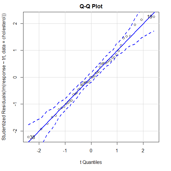
评估检验的假设条件
假设因变量服从正态分布,各组方差相等
Q-Q 图检验正态性假设
library(car)
qqPlot(
  lm(response ~ trt, data=cholesterol),
  simulate=TRUE,
  main="Q-Q Plot",
  labels=FALSE
)
[1] 19 38
方差齐性检验
Bartlett 检验
bartlett.test(
  response ~ trt,
  data=cholesterol
)
	Bartlett test of homogeneity of variances

data:  response by trt
Bartlett's K-squared = 0.57975, df = 4, p-value = 0.9653
Fligner-Killeen 检验
fligner.test(
  response ~ trt,
  data=cholesterol
)
	Fligner-Killeen test of homogeneity of variances

data:  response by trt
Fligner-Killeen:med chi-squared = 0.74277, df = 4, p-value = 0.946
Brown-Forsythe 检验
library(HH)
hov(
  response ~ trt,
  data=cholesterol
)
	hov: Brown-Forsyth

data:  response
F = 0.075477, df:trt = 4, df:Residuals = 45, p-value = 0.9893
alternative hypothesis: variances are not identical
car 包的 outlierTest() 函数检测离群点
outlierTest(fit)
No Studentized residuals with Bonferroni p < 0.05
Largest |rstudent|:
   rstudent unadjusted p-value Bonferroni p
19 2.251149           0.029422           NA
单因素协方差分析
ANCOVA
multcomp 包的 litter 数据集
head(litter)
  dose weight gesttime number
1    0  28.05     22.5     15
2    0  33.33     22.5     14
3    0  36.37     22.0     14
4    0  35.52     22.0     13
5    0  36.77     21.5     15
6    0  29.60     23.0      5
attach(litter)
table(dose)
dose
  0   5  50 500
 20  19  18  17
aggregate(
  weight,
  by=list(dose),
  FUN=mean
)
  Group.1        x
1       0 32.30850
2       5 29.30842
3      50 29.86611
4     500 29.64647
fit <- aov(
  weight ~ gesttime + dose
)
summary(fit)
            Df Sum Sq Mean Sq F value  Pr(>F)
gesttime     1  134.3  134.30   8.049 0.00597 **
dose         3  137.1   45.71   2.739 0.04988 *
Residuals   69 1151.3   16.69
---
Signif. codes:  0 ‘***’ 0.001 ‘**’ 0.01 ‘*’ 0.05 ‘.’ 0.1 ‘ ’ 1
effects 包中的 effect() 函数计算调整均值
library(effects)
effect("dose", fit)
 dose effect
dose
       0        5       50      500
32.35367 28.87672 30.56614 29.33460
multcomp 包的 glht() 函数
constrast <- rbind(
  "no drug vs. drug" = c(3, -1, -1, -1)
)
summary(
  glht(
    fit,
    linfct=mcp(dose=constrast)
  )
)
	 Simultaneous Tests for General Linear Hypotheses

Multiple Comparisons of Means: User-defined Contrasts


Fit: aov(formula = weight ~ gesttime + dose)

Linear Hypotheses:
                      Estimate Std. Error t value Pr(>|t|)
no drug vs. drug == 0    8.284      3.209   2.581    0.012 *
---
Signif. codes:  0 ‘***’ 0.001 ‘**’ 0.01 ‘*’ 0.05 ‘.’ 0.1 ‘ ’ 1
(Adjusted p values reported -- single-step method)
评估检验的假设条件
ANCOVA 需要正态性和同方差性假设,同时还假定回归效率相同
fit2 <- aov(
  weight ~ gesttime*dose,
  data=litter
)
summary(fit2)
              Df Sum Sq Mean Sq F value  Pr(>F)
gesttime       1  134.3  134.30   8.289 0.00537 **
dose           3  137.1   45.71   2.821 0.04556 *
gesttime:dose  3   81.9   27.29   1.684 0.17889
Residuals     66 1069.4   16.20
---
Signif. codes:  0 ‘***’ 0.001 ‘**’ 0.01 ‘*’ 0.05 ‘.’ 0.1 ‘ ’ 1
交互项不显著,支持斜率相等的假设
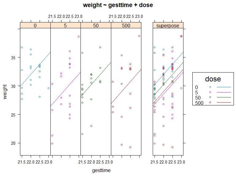
结果可视化
HH 包中的 ancova() 函数
library(HH)
ancova(
  weight ~ gesttime + dose,
  data=litter
)
Analysis of Variance Table

Response: weight
          Df  Sum Sq Mean Sq F value   Pr(>F)
gesttime   1  134.30 134.304  8.0493 0.005971 **
dose       3  137.12  45.708  2.7394 0.049883 *
Residuals 69 1151.27  16.685
---
Signif. codes:  0 ‘***’ 0.001 ‘**’ 0.01 ‘*’ 0.05 ‘.’ 0.1 ‘ ’ 1
detach(litter)
双因素方差分析
head(ToothGrowth)
   len supp dose
1  4.2   VC  0.5
2 11.5   VC  0.5
3  7.3   VC  0.5
4  5.8   VC  0.5
5  6.4   VC  0.5
6 10.0   VC  0.5
attach(ToothGrowth)
table(supp, dose)
    dose
supp 0.5  1  2
  OJ  10 10 10
  VC  10 10 10
aggregate(
  len,
  by=list(supp, dose),
  FUN=mean
)
  Group.1 Group.2     x
1      OJ     0.5 13.23
2      VC     0.5  7.98
3      OJ     1.0 22.70
4      VC     1.0 16.77
5      OJ     2.0 26.06
6      VC     2.0 26.14
aggregate(
  len,
  by=list(supp, dose),
  FUN=sd
)
  Group.1 Group.2        x
1      OJ     0.5 4.459709
2      VC     0.5 2.746634
3      OJ     1.0 3.910953
4      VC     1.0 2.515309
5      OJ     2.0 2.655058
6      VC     2.0 4.797731
dose <- factor(dose)
fit <- aov(len ~ supp*dose)
summary(fit)
            Df Sum Sq Mean Sq F value   Pr(>F)
supp         1  205.4   205.4  15.572 0.000231 ***
dose         2 2426.4  1213.2  92.000  < 2e-16 ***
supp:dose    2  108.3    54.2   4.107 0.021860 *
Residuals   54  712.1    13.2
---
Signif. codes:  0 ‘***’ 0.001 ‘**’ 0.01 ‘*’ 0.05 ‘.’ 0.1 ‘ ’ 1
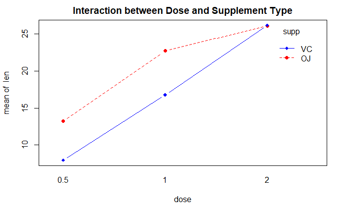
interaction.plot(
  dose, supp, len,
  type="b",
  col=c("red", "blue"),
  pch=c(16, 18),
  main="Interaction between Dose and Supplement Type"
)
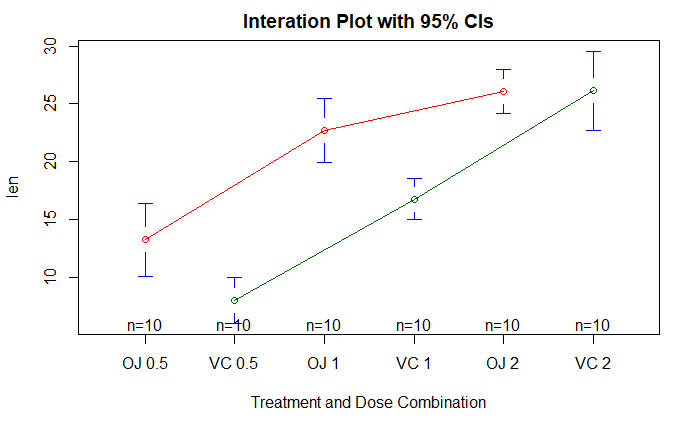
gplots 包中的 plotmeans() 函数展示交互作用
plotmeans(
  len ~ interaction(supp, dose, sep=" "),
  connect=list(c(1, 3, 5), c(2, 4, 6)),
  col=c("red", "darkgreen"),
  main="Interation Plot with 95% CIs",
  xlab="Treatment and Dose Combination"
)
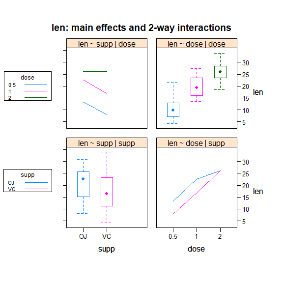
HH 包的 interaction2wt() 函数,对任意顺序的因子设计主效应和交互效应
interaction2wt(len ~ supp*dose, data=ToothGrowth)
重复测量方差分析
head(CO2)
Grouped Data: uptake ~ conc | Plant
  Plant   Type  Treatment conc uptake
1   Qn1 Quebec nonchilled   95   16.0
2   Qn1 Quebec nonchilled  175   30.4
3   Qn1 Quebec nonchilled  250   34.8
4   Qn1 Quebec nonchilled  350   37.2
5   Qn1 Quebec nonchilled  500   35.3
6   Qn1 Quebec nonchilled  675   39.2
CO2$conc <- factor(CO2$conc)
w1b1 <- subset(CO2, Treatment=="chilled")
head(w1b1)
Grouped Data: uptake ~ conc | Plant
   Plant   Type Treatment conc uptake
22   Qc1 Quebec   chilled   95   14.2
23   Qc1 Quebec   chilled  175   24.1
24   Qc1 Quebec   chilled  250   30.3
25   Qc1 Quebec   chilled  350   34.6
26   Qc1 Quebec   chilled  500   32.5
27   Qc1 Quebec   chilled  675   35.4
table(w1b1$Plant)
Qc1 Qc3 Qc2 Mc2 Mc3 Mc1
  7   7   7   7   7   7
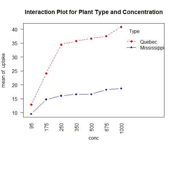
含一个组间因子(Type)和一个组内因子(conc)的重复测量方差分析
自变量:conc 和 Type
因变量:uptake
标识变量:Plant,表示重复测量
fit <- aov(
  uptake ~ conc * Type + Error(Plant/(conc)),
  w1b1
)
summary(fit)
Error: Plant
          Df Sum Sq Mean Sq F value  Pr(>F)
Type       1 2667.2  2667.2   60.41 0.00148 **
Residuals  4  176.6    44.1
---
Signif. codes:  0 ‘***’ 0.001 ‘**’ 0.01 ‘*’ 0.05 ‘.’ 0.1 ‘ ’ 1

Error: Plant:conc
          Df Sum Sq Mean Sq F value   Pr(>F)
conc       6 1472.4  245.40   52.52 1.26e-12 ***
conc:Type  6  428.8   71.47   15.30 3.75e-07 ***
Residuals 24  112.1    4.67
---
Signif. codes:  0 ‘***’ 0.001 ‘**’ 0.01 ‘*’ 0.05 ‘.’ 0.1 ‘ ’ 1
par(las=2)
par(mar=c(10, 4, 4, 2))
with(
  w1b1,
  interaction.plot(
    conc, Type, uptake,
    type="b",
    col=c("red", "blue"),
    pch=c(16, 18),
    main="Interaction Plot for Plant Type and Concentration"
  )
)
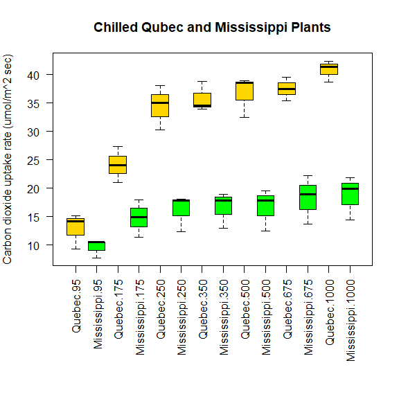
par(las=2)
par(mar=c(10, 4, 4, 2))
boxplot(
  uptake ~ Type*conc,
  data=w1b1,
  col=c("gold", "green"),
  main="Chilled Qubec and Mississippi Plants",
  ylab="Carbon dioxide uptake rate (umol/m^2 sec)",
  xlab=""
)
宽格式 wide format
列是变量,行是观测,一行一个受试对象
head(litter)
  dose weight gesttime number
1    0  28.05     22.5     15
2    0  33.33     22.5     14
3    0  36.37     22.0     14
4    0  35.52     22.0     13
5    0  36.77     21.5     15
6    0  29.60     23.0      5
长格式 long format
因变量的每次观测放到独立的行中
head(CO2)
Grouped Data: uptake ~ conc | Plant
  Plant   Type  Treatment conc uptake
1   Qn1 Quebec nonchilled   95   16.0
2   Qn1 Quebec nonchilled  175   30.4
3   Qn1 Quebec nonchilled  250   34.8
4   Qn1 Quebec nonchilled  350   37.2
5   Qn1 Quebec nonchilled  500   35.3
6   Qn1 Quebec nonchilled  675   39.2
多元方差分析
MANOVA
MASS 库的 UScereal 数据集
library(MASS)
head(UScereal)
                          mfr calories   protein      fat   sodium     fibre    carbo
100% Bran                   N 212.1212 12.121212 3.030303 393.9394 30.303030 15.15152
All-Bran                    K 212.1212 12.121212 3.030303 787.8788 27.272727 21.21212
All-Bran with Extra Fiber   K 100.0000  8.000000 0.000000 280.0000 28.000000 16.00000
Apple Cinnamon Cheerios     G 146.6667  2.666667 2.666667 240.0000  2.000000 14.00000
Apple Jacks                 K 110.0000  2.000000 0.000000 125.0000  1.000000 11.00000
Basic 4                     G 173.3333  4.000000 2.666667 280.0000  2.666667 24.00000
                            sugars shelf potassium vitamins
100% Bran                 18.18182     3 848.48485 enriched
All-Bran                  15.15151     3 969.69697 enriched
All-Bran with Extra Fiber  0.00000     3 660.00000 enriched
Apple Cinnamon Cheerios   13.33333     1  93.33333 enriched
Apple Jacks               14.00000     2  30.00000 enriched
Basic 4                   10.66667     3 133.33333 enriched
attach(UScereal)
shelf <- factor(shelf)
y <- cbind(
  calories, fat, sugars
)
head(y)
     calories      fat   sugars
[1,] 212.1212 3.030303 18.18182
[2,] 212.1212 3.030303 15.15151
[3,] 100.0000 0.000000  0.00000
[4,] 146.6667 2.666667 13.33333
[5,] 110.0000 0.000000 14.00000
[6,] 173.3333 2.666667 10.66667
aggregate(
  y,
  by=list(shelf),
  FUN=mean
)
  Group.1 calories       fat    sugars
1       1 119.4774 0.6621338  6.295493
2       2 129.8162 1.3413488 12.507670
3       3 180.1466 1.9449071 10.856821
cov(y)
           calories       fat     sugars
calories 3895.24210 60.674383 180.380317
fat        60.67438  2.713399   3.995474
sugars    180.38032  3.995474  34.050018
manova() 对组间差异进行多元检验
fit <- manova(y ~ shelf)
summary(fit)
          Df Pillai approx F num Df den Df    Pr(>F)
shelf      2 0.4021   5.1167      6    122 0.0001015 ***
Residuals 62
---
Signif. codes:  0 ‘***’ 0.001 ‘**’ 0.01 ‘*’ 0.05 ‘.’ 0.1 ‘ ’ 1
summary.aov() 函数对每一个变量做单因素方差分析
summary.aov(fit)
 Response calories :
            Df Sum Sq Mean Sq F value    Pr(>F)
shelf        2  50435 25217.6  7.8623 0.0009054 ***
Residuals   62 198860  3207.4
---
Signif. codes:  0 ‘***’ 0.001 ‘**’ 0.01 ‘*’ 0.05 ‘.’ 0.1 ‘ ’ 1

 Response fat :
            Df Sum Sq Mean Sq F value  Pr(>F)
shelf        2  18.44  9.2199  3.6828 0.03081 *
Residuals   62 155.22  2.5035
---
Signif. codes:  0 ‘***’ 0.001 ‘**’ 0.01 ‘*’ 0.05 ‘.’ 0.1 ‘ ’ 1

 Response sugars :
            Df  Sum Sq Mean Sq F value   Pr(>F)
shelf        2  381.33 190.667  6.5752 0.002572 **
Residuals   62 1797.87  28.998
---
Signif. codes:  0 ‘***’ 0.001 ‘**’ 0.01 ‘*’ 0.05 ‘.’ 0.1 ‘ ’ 1
评估假设检验
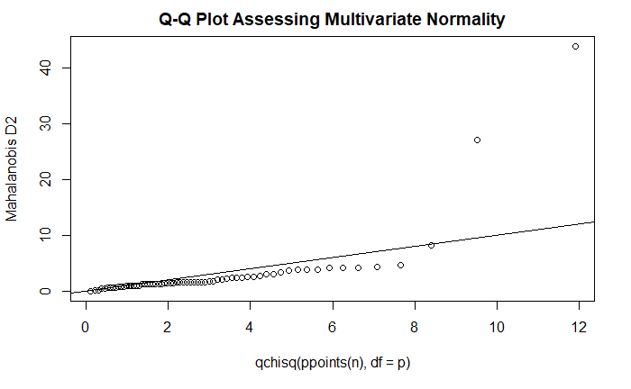
多元正态性
方差-协方差矩阵同质性
多元正态性:Q-Q 图
center <- colMeans(y)
cov <- cov(y)
d <- mahalanobis(y, center, cov)
n <- nrow(y)
p <- ncol(y)
coord <- qqplot(
  qchisq(
    ppoints(n),
    df=p
  ),
  d,
  main="Q-Q Plot Assessing Multivariate Normality",
  ylab="Mahalanobis D2"
)
abline(a=0, b=1)
方差-协方差同质性:Box’s M 检验
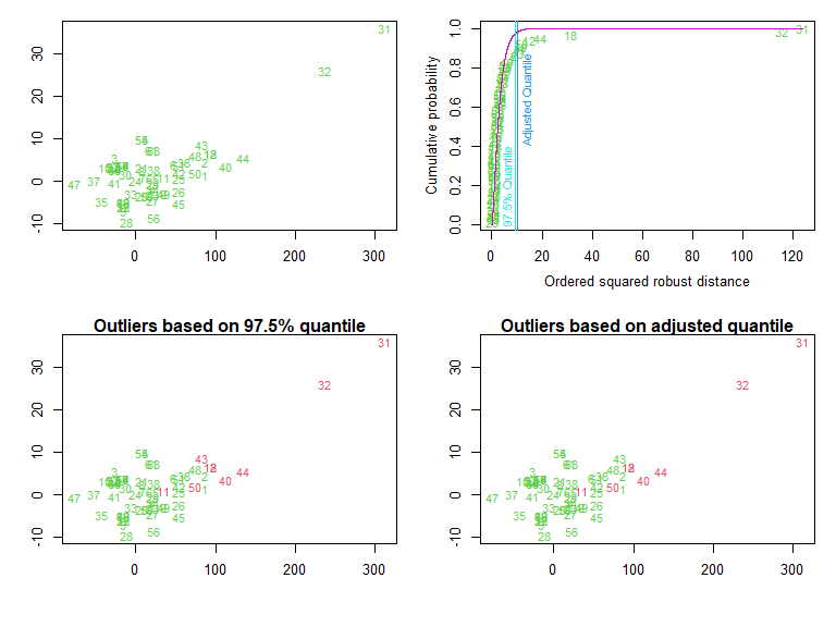
多元离群点:mvoutlier 包中的 ap.plot() 函数
library(mvoutlier)
outliers <- aq.plot(y)
outliers
稳健多元方差分析
稳健单因素 MANOVA:rrcov 包中的 Wilks.test() 函数
非参数 MANOVA:vegan 包中的 adonis() 函数
library(rrcov)
Wilks.test(
  y,
  shelf,
  method="mcd"
)
	Robust One-way MANOVA (Bartlett Chi2)

data:  x
Wilks' Lambda = 0.51073, Chi2-Value = 21.979, DF = 4.575, p-value = 0.0003573
sample estimates:
  calories       fat    sugars
1 119.8210 0.7010828  5.663143
2 128.0407 1.1849576 12.537533
3 160.8604 1.6524559 10.352646
用回归来做 ANOVA
levels(cholesterol$trt)
[1] "1time" "2times" "4times" "drugD" "drugE"
fit_aov <- aov(
  response ~ trt,
  data=cholesterol
)
summary(fit_aov)
            Df Sum Sq Mean Sq F value   Pr(>F)
trt          4 1351.4   337.8   32.43 9.82e-13 ***
Residuals   45  468.8    10.4
---
Signif. codes:  0 ‘***’ 0.001 ‘**’ 0.01 ‘*’ 0.05 ‘.’ 0.1 ‘ ’ 1
fit_lm <- lm(
  response ~ trt,
  data=cholesterol
)
summary(fit_lm)
Call:
lm(formula = response ~ trt, data = cholesterol)

Residuals:
    Min      1Q  Median      3Q     Max
-6.5418 -1.9672 -0.0016  1.8901  6.6008

Coefficients:
            Estimate Std. Error t value Pr(>|t|)
(Intercept)    5.782      1.021   5.665 9.78e-07 ***
trt2times      3.443      1.443   2.385   0.0213 *
trt4times      6.593      1.443   4.568 3.82e-05 ***
trtdrugD       9.579      1.443   6.637 3.53e-08 ***
trtdrugE      15.166      1.443  10.507 1.08e-13 ***
---
Signif. codes:  0 ‘***’ 0.001 ‘**’ 0.01 ‘*’ 0.05 ‘.’ 0.1 ‘ ’ 1

Residual standard error: 3.227 on 45 degrees of freedom
Multiple R-squared:  0.7425,	Adjusted R-squared:  0.7196
F-statistic: 32.43 on 4 and 45 DF,  p-value: 9.819e-13
contrasts(cholesterol$trt)
       2times 4times drugD drugE
1time       0      0     0     0
2times      1      0     0     0
4times      0      1     0     0
drugD       0      0     1     0
drugE       0      0     0     1
fit_lm <- lm(
  response ~ trt,
  data=cholesterol,
  contrasts=c("contr.SAS", "contr.helmert")
)
summary(fit_lm)
non-list contrasts argument ignored
Call:
lm(formula = response ~ trt, data = cholesterol, contrasts = c("contr.SAS",
    "contr.helmert"))

Residuals:
    Min      1Q  Median      3Q     Max
-6.5418 -1.9672 -0.0016  1.8901  6.6008

Coefficients:
            Estimate Std. Error t value Pr(>|t|)
(Intercept)    5.782      1.021   5.665 9.78e-07 ***
trt2times      3.443      1.443   2.385   0.0213 *
trt4times      6.593      1.443   4.568 3.82e-05 ***
trtdrugD       9.579      1.443   6.637 3.53e-08 ***
trtdrugE      15.166      1.443  10.507 1.08e-13 ***
---
Signif. codes:  0 ‘***’ 0.001 ‘**’ 0.01 ‘*’ 0.05 ‘.’ 0.1 ‘ ’ 1

Residual standard error: 3.227 on 45 degrees of freedom
Multiple R-squared:  0.7425,	Adjusted R-squared:  0.7196
F-statistic: 32.43 on 4 and 45 DF,  p-value: 9.819e-13
参考
https://github.com/perillaroc/r-in-action-study
R 语言实战
《图形初阶》
《基本数据管理》
《高级数据管理》
《基本图形》
《基本统计分析》
《回归》
