R语言实战:回归
本文内容来自《R 语言实战》(R in Action, 2nd),有部分修改
回归的多面性
- 简单线性
- 多项式
- 多层
- 多元线性
- 多变量
- Logistic
- 泊松
- Cox比例风险
- 时间序列
- 非线性
- 非参数
- 稳健
普通最小二乘 (OLS) 回归法,包括简单线性回归,多项式回归和多元线性回归。
OLS 回归的适用情景
- 发现有趣的问题
- 设计一个有用的、可以测量的响应变量
- 收集合适的数据
基础回顾
OLS 回归
$$ \hat{Y_i}=\hat{\beta_0} + \hat{\beta_1}X_{1i} + … + \hat{\beta_k}X_{ki} $$
残差平方和最小
$$ \sum_{i=1}^{n}(Y_i-\hat{Y_i})^2=\sum_{i=1}^{n}(Y_i-\hat{\beta_0}+\hat{\beta_1}X_{1i}+…+\hat{\beta_k}X_{ki})=\sum_{i=1}^{n}\epsilon_i^2 $$
统计假设
- 正态性:对于固定的自变量值,因变量值成正态分布
- 独立性:Y_i 值之间相互独立
- 线性:因变量与自变量之间为线性相关
- 同方差性:因变量的方差不随自变量的水平不同而变化
用 lm() 拟合回归模型
简单线性回归
多项式回归
多元线性回归
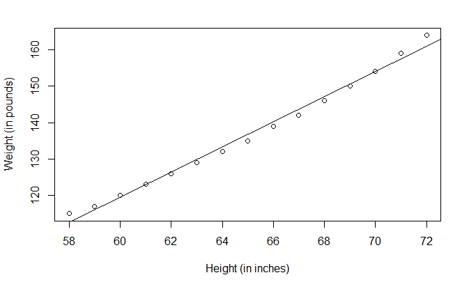
简单线性回归
数据集
head(women)
  height weight
1     58    115
2     59    117
3     60    120
4     61    123
5     62    126
6     63    129
summary() 函数
fit <- lm(
  weight ~ height,
  data=women
)
summary(fit)
Call:
lm(formula = weight ~ height, data = women)

Residuals:
    Min      1Q  Median      3Q     Max
-1.7333 -1.1333 -0.3833  0.7417  3.1167

Coefficients:
             Estimate Std. Error t value Pr(>|t|)
(Intercept) -87.51667    5.93694  -14.74 1.71e-09 ***
height        3.45000    0.09114   37.85 1.09e-14 ***
---
Signif. codes:  0 ‘***’ 0.001 ‘**’ 0.01 ‘*’ 0.05 ‘.’ 0.1 ‘ ’ 1

Residual standard error: 1.525 on 13 degrees of freedom
Multiple R-squared:  0.991,	Adjusted R-squared:  0.9903
F-statistic:  1433 on 1 and 13 DF,  p-value: 1.091e-14
目标值
women$weight
[1] 115 117 120 123 126 129 132 135 139 142 146 150 154 159 164
fitted() 函数计算预测值
fitted(fit)
       1        2        3        4        5        6        7        8        9       10       11       12
112.5833 116.0333 119.4833 122.9333 126.3833 129.8333 133.2833 136.7333 140.1833 143.6333 147.0833 150.5333
      13       14       15
153.9833 157.4333 160.8833
residuals() 函数返回残差
residuals(fit)
          1           2           3           4           5           6           7           8           9
 2.41666667  0.96666667  0.51666667  0.06666667 -0.38333333 -0.83333333 -1.28333333 -1.73333333 -1.18333333
         10          11          12          13          14          15
-1.63333333 -1.08333333 -0.53333333  0.01666667  1.56666667  3.11666667
abline() 绘制拟合直线
plot(
  women$height,
  women$weight,
  xlab="Height (in inches)",
  ylab="Weight (in pounds)"
)
abline(fit)
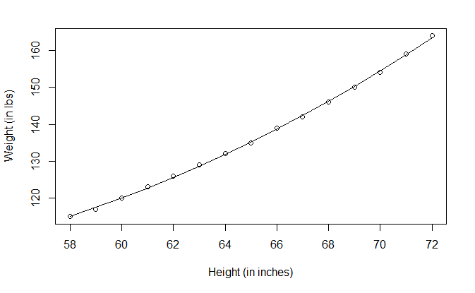
多项式回归
fit2 <- lm(
  weight ~ height + I(height^2),
  data=women
)
summary(fit2)
Call:
lm(formula = weight ~ height + I(height^2), data = women)

Residuals:
     Min       1Q   Median       3Q      Max
-0.50941 -0.29611 -0.00941  0.28615  0.59706

Coefficients:
             Estimate Std. Error t value Pr(>|t|)
(Intercept) 261.87818   25.19677  10.393 2.36e-07 ***
height       -7.34832    0.77769  -9.449 6.58e-07 ***
I(height^2)   0.08306    0.00598  13.891 9.32e-09 ***
---
Signif. codes:  0 ‘***’ 0.001 ‘**’ 0.01 ‘*’ 0.05 ‘.’ 0.1 ‘ ’ 1

Residual standard error: 0.3841 on 12 degrees of freedom
Multiple R-squared:  0.9995,	Adjusted R-squared:  0.9994
F-statistic: 1.139e+04 on 2 and 12 DF,  p-value: < 2.2e-16
plot(
  women$height,
  women$weight,
  xlab="Height (in inches)",
  ylab="Weight (in lbs)"
)
lines(women$height, fitted(fit2))
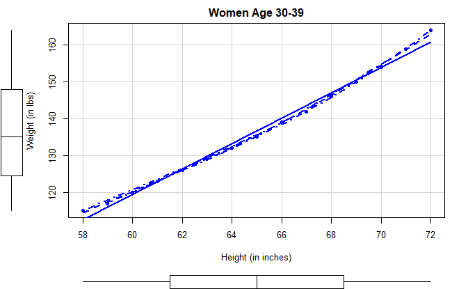
car 包的 scatterplot() 函数
library(car)
scatterplot(
  weight ~ height,
  data=women,
  smooth=list(lty=2),
  pch=19,
  main="Women Age 30-39",
  xlab="Height (in inches)",
  ylab="Weight (in lbs)"
)
多元线性回归
head(state.x77)
           Population Income Illiteracy Life Exp Murder HS Grad Frost   Area
Alabama          3615   3624        2.1    69.05   15.1    41.3    20  50708
Alaska            365   6315        1.5    69.31   11.3    66.7   152 566432
Arizona          2212   4530        1.8    70.55    7.8    58.1    15 113417
Arkansas         2110   3378        1.9    70.66   10.1    39.9    65  51945
California      21198   5114        1.1    71.71   10.3    62.6    20 156361
Colorado         2541   4884        0.7    72.06    6.8    63.9   166 103766
states <- as.data.frame(
  state.x77[,c(
    "Murder",
    "Population",
    "Illiteracy",
    "Income",
    "Frost"
  )]
)
head(states)
           Murder Population Illiteracy Income Frost
Alabama      15.1       3615        2.1   3624    20
Alaska       11.3        365        1.5   6315   152
Arizona       7.8       2212        1.8   4530    15
Arkansas     10.1       2110        1.9   3378    65
California   10.3      21198        1.1   5114    20
Colorado      6.8       2541        0.7   4884   166
cor() 检查相关性
cor(states)
               Murder Population Illiteracy     Income      Frost
Murder      1.0000000  0.3436428  0.7029752 -0.2300776 -0.5388834
Population  0.3436428  1.0000000  0.1076224  0.2082276 -0.3321525
Illiteracy  0.7029752  0.1076224  1.0000000 -0.4370752 -0.6719470
Income     -0.2300776  0.2082276 -0.4370752  1.0000000  0.2262822
Frost      -0.5388834 -0.3321525 -0.6719470  0.2262822  1.0000000
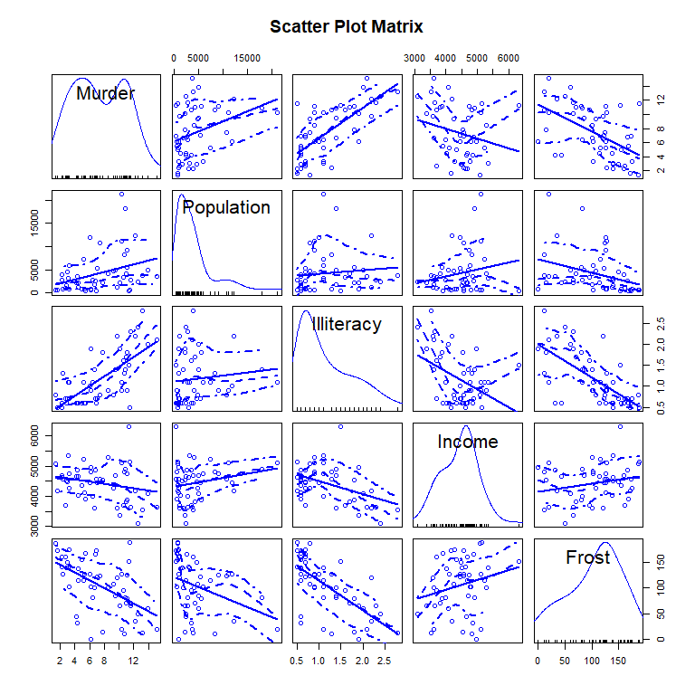
car 包的 scatterplotMatrix() 函数
scatterplotMatrix(
  states,
  smooth=list(lty=2),
  main="Scatter Plot Matrix"
)
fit_multi <- lm(
  Murder ~ Population + Illiteracy + Income + Frost,
  data=states
)
summary(fit_multi)
Call:
lm(formula = Murder ~ Population + Illiteracy + Income + Frost,
    data = states)

Residuals:
    Min      1Q  Median      3Q     Max
-4.7960 -1.6495 -0.0811  1.4815  7.6210

Coefficients:
             Estimate Std. Error t value Pr(>|t|)
(Intercept) 1.235e+00  3.866e+00   0.319   0.7510
Population  2.237e-04  9.052e-05   2.471   0.0173 *
Illiteracy  4.143e+00  8.744e-01   4.738 2.19e-05 ***
Income      6.442e-05  6.837e-04   0.094   0.9253
Frost       5.813e-04  1.005e-02   0.058   0.9541
---
Signif. codes:  0 ‘***’ 0.001 ‘**’ 0.01 ‘*’ 0.05 ‘.’ 0.1 ‘ ’ 1

Residual standard error: 2.535 on 45 degrees of freedom
Multiple R-squared:  0.567,	Adjusted R-squared:  0.5285
F-statistic: 14.73 on 4 and 45 DF,  p-value: 9.133e-08
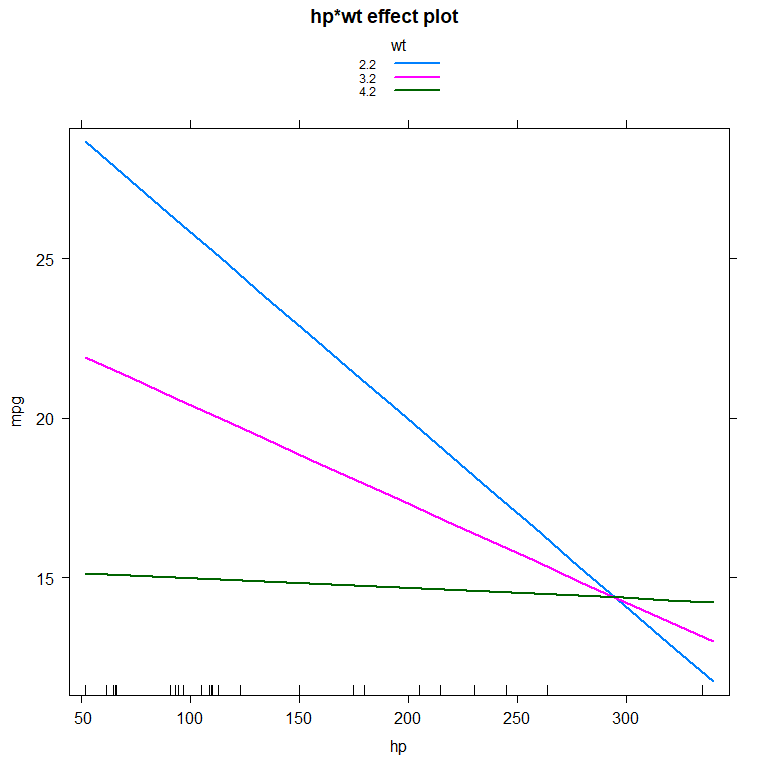
有交互项的多元线性回归
fit_inter <- lm(
  mpg ~ hp + wt + hp:wt,
  data=mtcars
)
summary(fit_inter)
Call:
lm(formula = mpg ~ hp + wt + hp:wt, data = mtcars)

Residuals:
    Min      1Q  Median      3Q     Max
-3.0632 -1.6491 -0.7362  1.4211  4.5513

Coefficients:
            Estimate Std. Error t value Pr(>|t|)
(Intercept) 49.80842    3.60516  13.816 5.01e-14 ***
hp          -0.12010    0.02470  -4.863 4.04e-05 ***
wt          -8.21662    1.26971  -6.471 5.20e-07 ***
hp:wt        0.02785    0.00742   3.753 0.000811 ***
---
Signif. codes:  0 ‘***’ 0.001 ‘**’ 0.01 ‘*’ 0.05 ‘.’ 0.1 ‘ ’ 1

Residual standard error: 2.153 on 28 degrees of freedom
Multiple R-squared:  0.8848,	Adjusted R-squared:  0.8724
F-statistic: 71.66 on 3 and 28 DF,  p-value: 2.981e-13
effects 包中的 effect() 函数
library(effects)
展示 wt 取 3 个值时,mpg 和 hp 的关系
plot(
  effect(
    "hp:wt",
    fit_inter,
    xlevels=list(
      wt=c(2.2, 3.2, 4.2)
    )
  ),
  multiline=TRUE
)
回归诊断
confint() 函数
confint(fit_multi)
                    2.5 %       97.5 %
(Intercept) -6.552191e+00 9.0213182149
Population   4.136397e-05 0.0004059867
Illiteracy   2.381799e+00 5.9038743192
Income      -1.312611e-03 0.0014414600
Frost       -1.966781e-02 0.0208304170
回归诊断技术
标准方法
fit <- lm(
  weight ~ height,
  data=women
)
summary(fit)
Call:
lm(formula = weight ~ height, data = women)

Residuals:
    Min      1Q  Median      3Q     Max
-1.7333 -1.1333 -0.3833  0.7417  3.1167

Coefficients:
             Estimate Std. Error t value Pr(>|t|)
(Intercept) -87.51667    5.93694  -14.74 1.71e-09 ***
height        3.45000    0.09114   37.85 1.09e-14 ***
---
Signif. codes:  0 ‘***’ 0.001 ‘**’ 0.01 ‘*’ 0.05 ‘.’ 0.1 ‘ ’ 1

Residual standard error: 1.525 on 13 degrees of freedom
Multiple R-squared:  0.991,	Adjusted R-squared:  0.9903
F-statistic:  1433 on 1 and 13 DF,  p-value: 1.091e-14
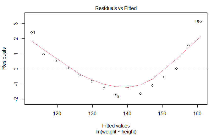
plot() 函数生成 4 幅图
plot(fit)
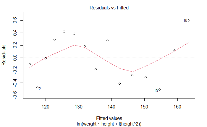
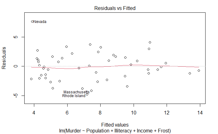
残差与拟合图
Residuals vs Fitted
线性。如果满足,残差值与拟合值没有任何关联
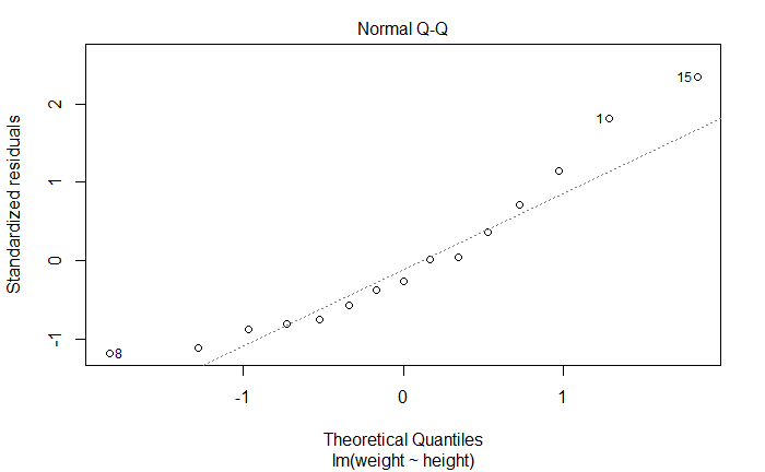
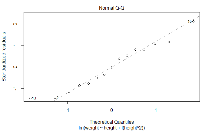
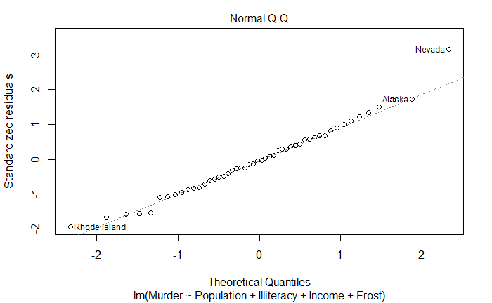
正态 Q-Q 图
Normal Q-Q
正态性。如果满足,残差值应该是均值为 0 的正态分布,沿 45 度角直线分布
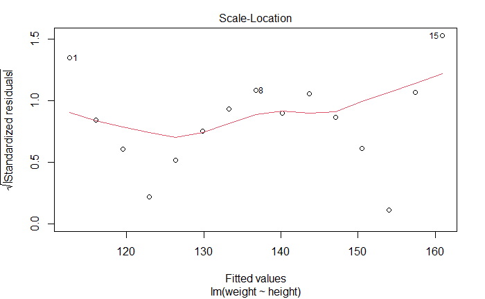
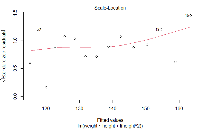
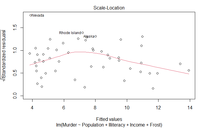
位置尺度图
Scale-Location Graph
同方差性。如果满足,水平线周围点应该随机分布
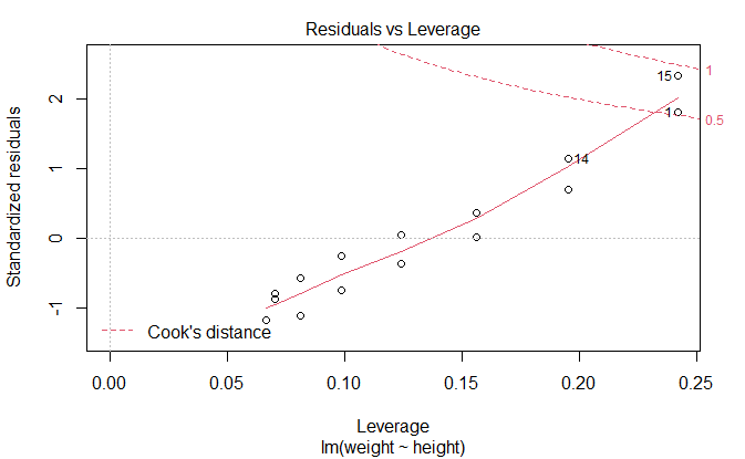
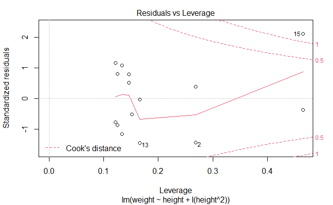
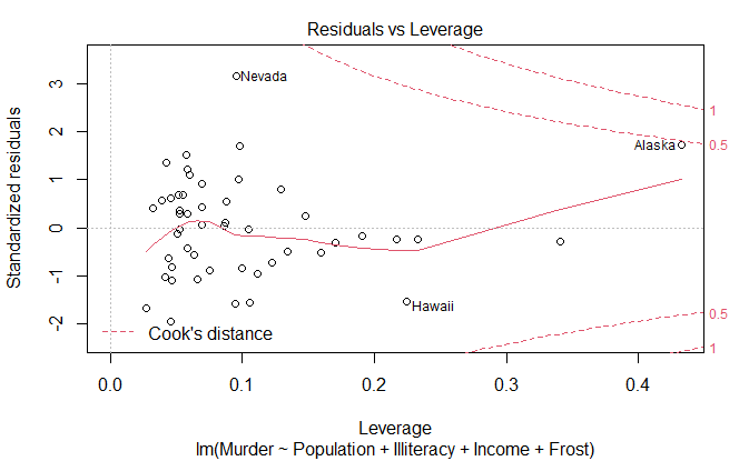
残差与杠杆图
Residuals vs Leverage
鉴别离群点,杠杆点和强影响点
fit2 <- lm(
  weight ~ height + I(height^2),
  data=women
)
summary(fit2)
Call:
lm(formula = weight ~ height + I(height^2), data = women)

Residuals:
     Min       1Q   Median       3Q      Max
-0.50941 -0.29611 -0.00941  0.28615  0.59706

Coefficients:
             Estimate Std. Error t value Pr(>|t|)
(Intercept) 261.87818   25.19677  10.393 2.36e-07 ***
height       -7.34832    0.77769  -9.449 6.58e-07 ***
I(height^2)   0.08306    0.00598  13.891 9.32e-09 ***
---
Signif. codes:  0 ‘***’ 0.001 ‘**’ 0.01 ‘*’ 0.05 ‘.’ 0.1 ‘ ’ 1

Residual standard error: 0.3841 on 12 degrees of freedom
Multiple R-squared:  0.9995,	Adjusted R-squared:  0.9994
F-statistic: 1.139e+04 on 2 and 12 DF,  p-value: < 2.2e-16
plot(fit2)
newfit <- lm(
  weight ~ height + I(height^2),
  data=women[-c(13, 15)]
)
summary(newfit)
Call:
lm(formula = weight ~ height + I(height^2), data = women[-c(13,
    15)])

Residuals:
     Min       1Q   Median       3Q      Max
-0.50941 -0.29611 -0.00941  0.28615  0.59706

Coefficients:
             Estimate Std. Error t value Pr(>|t|)
(Intercept) 261.87818   25.19677  10.393 2.36e-07 ***
height       -7.34832    0.77769  -9.449 6.58e-07 ***
I(height^2)   0.08306    0.00598  13.891 9.32e-09 ***
---
Signif. codes:  0 ‘***’ 0.001 ‘**’ 0.01 ‘*’ 0.05 ‘.’ 0.1 ‘ ’ 1

Residual standard error: 0.3841 on 12 degrees of freedom
Multiple R-squared:  0.9995,	Adjusted R-squared:  0.9994
F-statistic: 1.139e+04 on 2 and 12 DF,  p-value: < 2.2e-16
fit <- lm(
  Murder ~ Population + Illiteracy + Income + Frost,
  data=states
)
summary(fit)
Call:
lm(formula = Murder ~ Population + Illiteracy + Income + Frost,
    data = states)

Residuals:
    Min      1Q  Median      3Q     Max
-4.7960 -1.6495 -0.0811  1.4815  7.6210

Coefficients:
             Estimate Std. Error t value Pr(>|t|)
(Intercept) 1.235e+00  3.866e+00   0.319   0.7510
Population  2.237e-04  9.052e-05   2.471   0.0173 *
Illiteracy  4.143e+00  8.744e-01   4.738 2.19e-05 ***
Income      6.442e-05  6.837e-04   0.094   0.9253
Frost       5.813e-04  1.005e-02   0.058   0.9541
---
Signif. codes:  0 ‘***’ 0.001 ‘**’ 0.01 ‘*’ 0.05 ‘.’ 0.1 ‘ ’ 1

Residual standard error: 2.535 on 45 degrees of freedom
Multiple R-squared:  0.567,	Adjusted R-squared:  0.5285
F-statistic: 14.73 on 4 and 45 DF,  p-value: 9.133e-08
plot(fit)
改进方法
car 包,gvlma 包
fit <- lm(
  Murder ~ Population + Illiteracy + Income + Frost,
  data=states
)
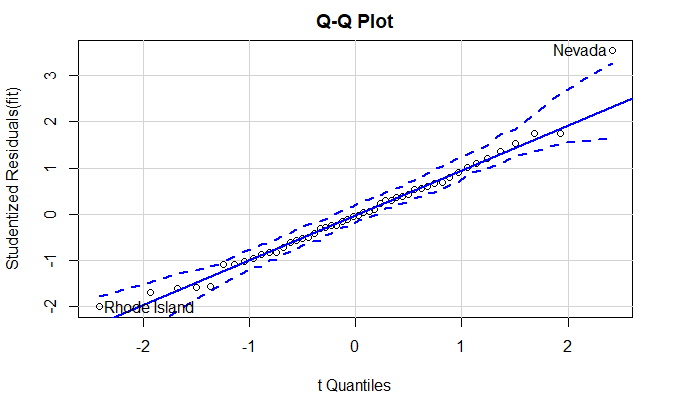
正态性
car::qqPlot()
qqPlot(
  fit,
  labels=row.names(states),
  id.method="identify",
  simulate=TRUE,
  main="Q-Q Plot"
)
      Nevada Rhode Island
          28           39
states["Nevada",]
       Murder Population Illiteracy Income Frost
Nevada   11.5        590        0.5   5149   188
fitted(fit)["Nevada"]
  Nevada
3.878958
residuals(fit)["Nevada"]
  Nevada
7.621042
rstudent(fit)["Nevada"]
  Nevada
3.542929
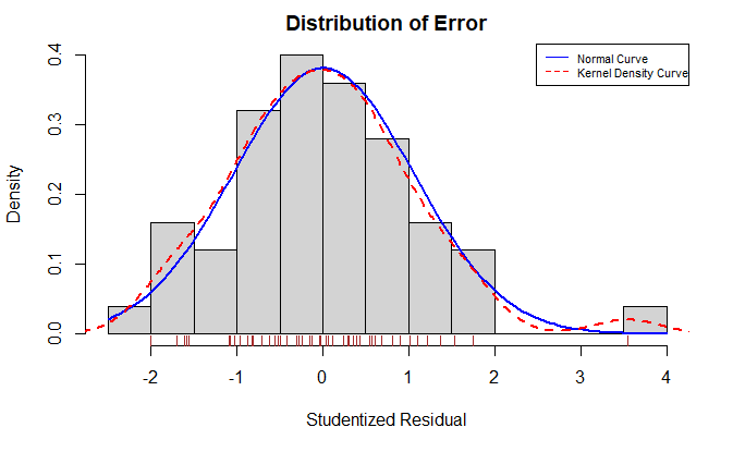
下面函数生成学生化残差的柱状图
residplot <- function(fit, nbreaks=10) {
  z <- rstudent(fit)
  hist(
    z,
    breaks=nbreaks,
    freq=FALSE,
    xlab="Studentized Residual",
    main="Distribution of Error"
  )
  rug(
    jitter(z),
    col="brown"
  )
  curve(
    dnorm(
      x,
      mean=mean(z),
      sd=sd(z)
    ),
    add=TRUE,
    col="blue",
    lwd=2
  )
  lines(
    density(z)$x,
    density(z)$y,
    col="red",
    lwd=2,
    lty=2
  )
  legend(
    "topright",
    legend=c("Normal Curve", "Kernel Density Curve"),
    lty=1:2,
    col=c("blue", "red"),
    cex=.7
  )
}
residplot(fit)
误差的独立性
Durbin-Watson 检验
car 包的 durbinWastsonTest() 函数
durbinWatsonTest(fit)
 lag Autocorrelation D-W Statistic p-value
   1      -0.2006929      2.317691   0.256
 Alternative hypothesis: rho != 0
p 不显著 (p=0.254),说明无自相关性,误差项之间独立
线性
成分残差图 component plus residual plot,偏残差图 partial residual plot
car 包的 crPlots() 函数
crPlots(fit)
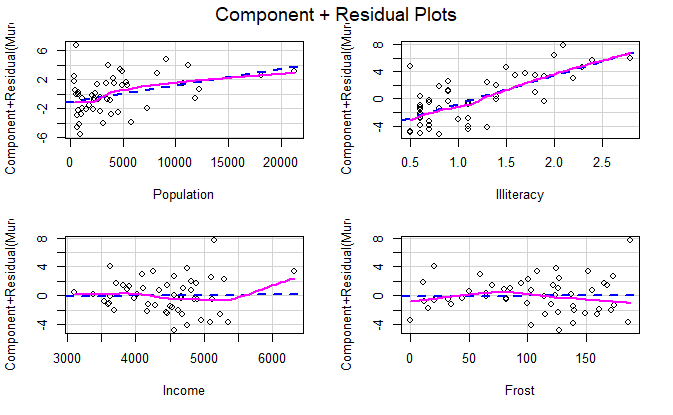
如果图形存在非线性,说明建模不够充分
同方差性
car 包的 ncvTest() 函数
零假设为误差方差不变
ncvTest(fit)
Non-constant Variance Score Test
Variance formula: ~ fitted.values
Chisquare = 1.746514, Df = 1, p = 0.18632
p 值不显著,说明满足零假设,即满足方差不变假设
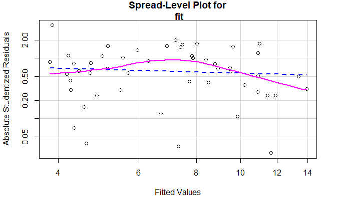
car 包的 spreadLevelPlot() 函数
spreadLevelPlot(fit)
Suggested power transformation: 1.209626
线性模型假设的综合验证
gvlma 包中的 gvlma() 函数
library(gvlma)
gvmodel <- gvlma(fit)
summary(gvmodel)
Call:
lm(formula = Murder ~ Population + Illiteracy + Income + Frost,
    data = states)

Residuals:
    Min      1Q  Median      3Q     Max
-4.7960 -1.6495 -0.0811  1.4815  7.6210

Coefficients:
             Estimate Std. Error t value Pr(>|t|)
(Intercept) 1.235e+00  3.866e+00   0.319   0.7510
Population  2.237e-04  9.052e-05   2.471   0.0173 *
Illiteracy  4.143e+00  8.744e-01   4.738 2.19e-05 ***
Income      6.442e-05  6.837e-04   0.094   0.9253
Frost       5.813e-04  1.005e-02   0.058   0.9541
---
Signif. codes:  0 ‘***’ 0.001 ‘**’ 0.01 ‘*’ 0.05 ‘.’ 0.1 ‘ ’ 1

Residual standard error: 2.535 on 45 degrees of freedom
Multiple R-squared:  0.567,	Adjusted R-squared:  0.5285
F-statistic: 14.73 on 4 and 45 DF,  p-value: 9.133e-08


ASSESSMENT OF THE LINEAR MODEL ASSUMPTIONS
USING THE GLOBAL TEST ON 4 DEGREES-OF-FREEDOM:
Level of Significance =  0.05

Call:
 gvlma(x = fit)

                    Value p-value                Decision
Global Stat        2.7728  0.5965 Assumptions acceptable.
Skewness           1.5374  0.2150 Assumptions acceptable.
Kurtosis           0.6376  0.4246 Assumptions acceptable.
Link Function      0.1154  0.7341 Assumptions acceptable.
Heteroscedasticity 0.4824  0.4873 Assumptions acceptable.
多重共线性
VIF,Variance Inflation Factor,方差膨胀因子
car 包的 vif() 函数
vif(fit)
Population Illiteracy     Income      Frost
  1.245282   2.165848   1.345822   2.082547
一般原则,\sqrt{vif} > 2 表明存在多重共线性问题
sqrt(vif(fit)) > 2
Population Illiteracy     Income      Frost
     FALSE      FALSE      FALSE      FALSE
异常观测值
离群点
粗糙判断的两种方法:
- Q-Q 图中落在置信区间带外的点
- 标准化残差值大于 2 或者小于 -2
car 包的 outlierTest() 函数
outlierTest(fit)
       rstudent unadjusted p-value Bonferroni p
Nevada 3.542929         0.00095088     0.047544
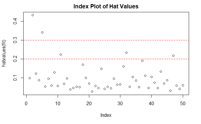
高杠杆点
帽子统计量,hat statistic
帽子值大于帽子均值的 2 或 3 倍,帽子均值为 p/n
hat.plot <- function(fit) {
  p <- length(coefficients(fit))
  n <- length(fitted(fit))
  plot(
    hatvalues(fit),
    main="Index Plot of Hat Values"
  )
  abline(
    h=c(2, 3)*p/n,
    col="red",
    lty=2
  )
}
hat.plot(fit)
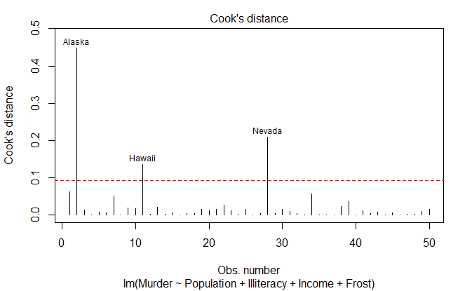
强影响点
两种检测方法:
- Cook 距离,D 统计量,大于
4/(n-k-1) - 变量添加图,added variable plot
cutoff <- 4 / (
  nrow(states) - length(fit$coefficients) - 2
)
plot(
  fit,
  which=4,
  cook.levels=cutoff
)
abline(
  h=cutoff,
  lty=2,
  col="red"
)
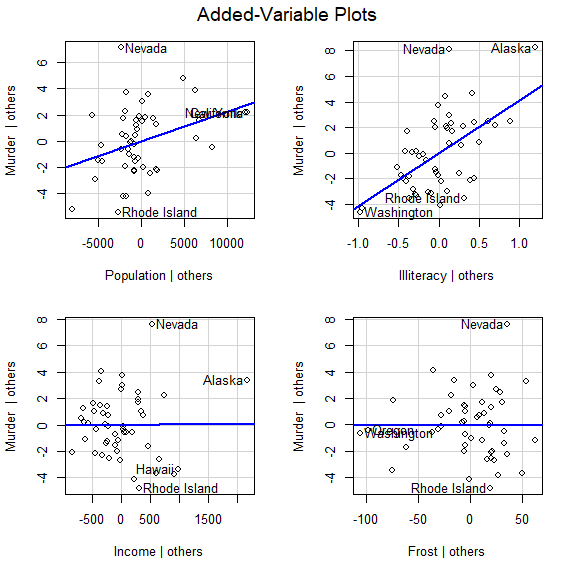
car 包的 avPlot() 函数
avPlots(
  fit,
  ask=FALSE
)
car 包的 influencePlot() 函数
influencePlot(
  fit,
  main="Influence Plot",
  sub="Circle size if proportional to Cook's distance"
)
                StudRes        Hat       CookD
Alaska        1.7536917 0.43247319 0.448050997
California   -0.2761492 0.34087628 0.008052956
Nevada        3.5429286 0.09508977 0.209915743
Rhode Island -2.0001631 0.04562377 0.035858963
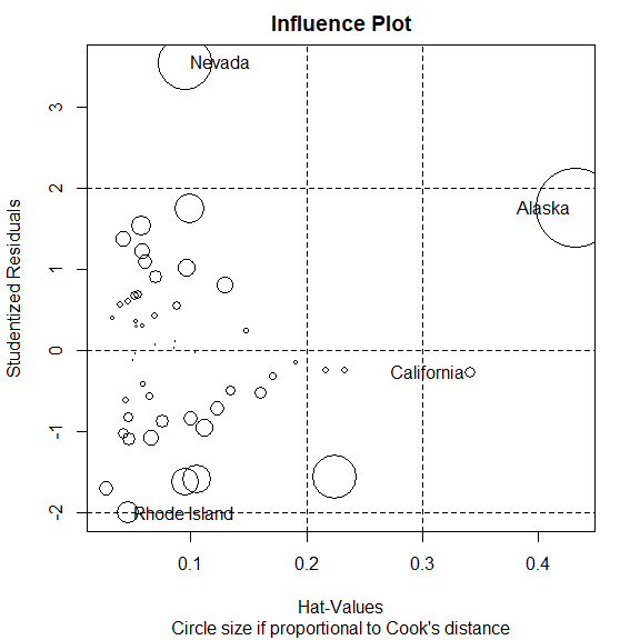
纵坐标大于 +2 或小于 -2 的点是离群点。
横坐标大于 0.2 或 0.3 的点是高杠杆点。
圆圈很大的点是强影响点。
改进措施
删除观测点
谨慎删除离群点和强影响点
变量变换
car 包的 powerTransform() 函数通过 lambda 的最大似然估计来正态化变量 X^{lambda}
summary(
  powerTransform(states$Murder)
)
bcPower Transformation to Normality
              Est Power Rounded Pwr Wald Lwr Bnd Wald Upr Bnd
states$Murder    0.6055           1       0.0884       1.1227

Likelihood ratio test that transformation parameter is equal to 0
 (log transformation)
                           LRT df     pval
LR test, lambda = (0) 5.665991  1 0.017297

Likelihood ratio test that no transformation is needed
                           LRT df    pval
LR test, lambda = (1) 2.122763  1 0.14512
car 包的 boxTidwell() 函数最大似然估计预测变量幂数
boxTidwell(
  Murder ~ Population + Illiteracy,
  data=states
)
           MLE of lambda Score Statistic (z) Pr(>|z|)
Population       0.86939             -0.3228   0.7468
Illiteracy       1.35812              0.6194   0.5357

iterations =  19
删增变量
删除变量方法举例:
- 删除某个多重共线性的变量
- 岭回归
尝试其他方法
存在离群点和/或强影响点:稳健回归模型
违背正态性假设:非参数回归模型
显著的非线性:非线性回归模型
违背误差独立性假设:时间序列模型,多层次回归模型。。。
广义线性模型
选择“最佳”的回归模型
模型比较
anova() 函数比较两个嵌套模型的拟合优度
fit1 <- lm(
  Murder ~ Population + Illiteracy + Income + Frost,
  data=states
)
fit2 <- lm(
  Murder ~ Population + Illiteracy,
  data=states
)

anova(fit2, fit1)
Analysis of Variance Table

Model 1: Murder ~ Population + Illiteracy
Model 2: Murder ~ Population + Illiteracy + Income + Frost
  Res.Df    RSS Df Sum of Sq      F Pr(>F)
1     47 289.25
2     45 289.17  2  0.078505 0.0061 0.9939
赤池信息准则(AIC,Akaike Information Criterion)
AIC 较小的模型优先选择
fit1 <- lm(
  Murder ~ Population + Illiteracy + Income + Frost,
  data=states
)
fit2 <- lm(
  Murder ~ Population + Illiteracy,
  data=states
)
AIC(fit1, fit2)
     df      AIC
fit1  6 241.6429
fit2  4 237.6565
变量选择
逐步回归法
stepwise method
向前逐步回归 forward stepwise regression
向后逐步回归 backward stepwise regression
向前向后逐步回归,逐步回归,stepwise stepwise regression
MASS 包中的 stepAIC() 函数
library(MASS)
fit <- lm(
  Murder ~ Population + Illiteracy + Income + Frost,
  data=states
)
stepAIC(fit, direction="backward")
Start:  AIC=97.75
Murder ~ Population + Illiteracy + Income + Frost

             Df Sum of Sq    RSS     AIC
- Frost       1     0.021 289.19  95.753
- Income      1     0.057 289.22  95.759
<none>                    289.17  97.749
- Population  1    39.238 328.41 102.111
- Illiteracy  1   144.264 433.43 115.986

Step:  AIC=95.75
Murder ~ Population + Illiteracy + Income

             Df Sum of Sq    RSS     AIC
- Income      1     0.057 289.25  93.763
<none>                    289.19  95.753
- Population  1    43.658 332.85 100.783
- Illiteracy  1   236.196 525.38 123.605

Step:  AIC=93.76
Murder ~ Population + Illiteracy

             Df Sum of Sq    RSS     AIC
<none>                    289.25  93.763
- Population  1    48.517 337.76  99.516
- Illiteracy  1   299.646 588.89 127.311

Call:
lm(formula = Murder ~ Population + Illiteracy, data = states)

Coefficients:
(Intercept)   Population   Illiteracy
  1.6515497    0.0002242    4.0807366
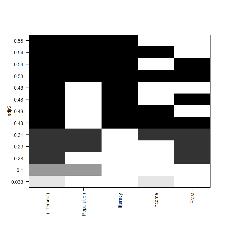
全子集回归
leaps 包的 regsubsets() 函数
R 平方
调整 R 平方
Mallows Cp 统计量
library(leaps)
leaps <- regsubsets(
  Murder ~ Population + Illiteracy + Income + Frost,
  data=states,
  nbest=4
)
summary(leaps)
Subset selection object
Call: regsubsets.formula(Murder ~ Population + Illiteracy + Income +
    Frost, data = states, nbest = 4)
4 Variables  (and intercept)
           Forced in Forced out
Population     FALSE      FALSE
Illiteracy     FALSE      FALSE
Income         FALSE      FALSE
Frost          FALSE      FALSE
4 subsets of each size up to 4
Selection Algorithm: exhaustive
         Population Illiteracy Income Frost
1  ( 1 ) " "        "*"        " "    " "
1  ( 2 ) " "        " "        " "    "*"
1  ( 3 ) "*"        " "        " "    " "
1  ( 4 ) " "        " "        "*"    " "
2  ( 1 ) "*"        "*"        " "    " "
2  ( 2 ) " "        "*"        " "    "*"
2  ( 3 ) " "        "*"        "*"    " "
2  ( 4 ) "*"        " "        " "    "*"
3  ( 1 ) "*"        "*"        "*"    " "
3  ( 2 ) "*"        "*"        " "    "*"
3  ( 3 ) " "        "*"        "*"    "*"
3  ( 4 ) "*"        " "        "*"    "*"
4  ( 1 ) "*"        "*"        "*"    "*"
每一行表示一个组合,变量是色块对应的横坐标
plot(leaps, scale="adjr2")
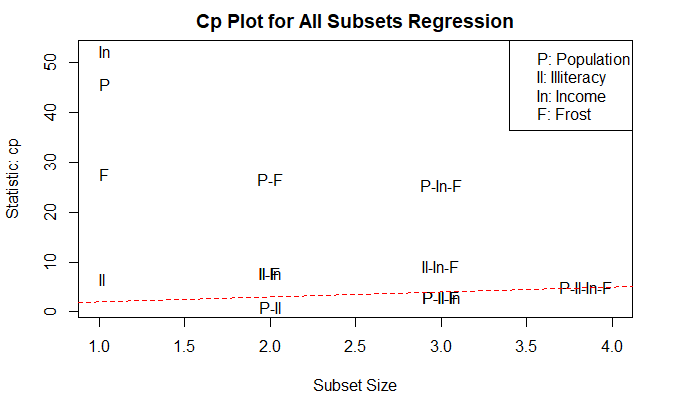
car 包的 subsets() 函数
越好的模型越接近直线
subsets(
  leaps,
  statistic="cp",
  main="Cp Plot for All Subsets Regression",
  legend="topright"
)
abline(
  1, 1,
  lty=2,
  col="red"
)
深层次分析
交叉验证
模型泛化能力
k 重交叉验证
bootstrap 包的 crossval() 函数
shrinkage <- function(fit, k=10) {
  require(bootstrap)
  theta.fit <- function(x, y)(lsfit(x, y))
  theta.predict <- function(fit, x){
    cbind(1, x)%*%fit$coefficients
  }

  x <- fit$model[, 2:ncol(fit$model)]
  y <- fit$model[, 1]

  results <- crossval(
    x, y,
    theta.fit,
    theta.predict,
    ngroup=k
  )

  r2 <- cor(
    y,
    fit$fitted.values
  )^2

  r2cv <- cor(
    y,
    results$cv.fit
  )^2

  cat("Original R-square =", r2, "\n")
  cat(k, "Fold Cross-Validated R-square = ", r2cv, "\n")
  cat("Change =", r2 - r2cv, "\n")
}
fit <- lm(
  Murder ~ Population + Income + Illiteracy + Frost,
  data=states
)
shrinkage(fit)
Original R-square = 0.5669502
10 Fold Cross-Validated R-square =  0.4707088
Change = 0.09624146
fit2 <- lm(
  Murder ~ Population + Illiteracy,
  data=states
)
shrinkage(fit2)
Original R-square = 0.5668327
10 Fold Cross-Validated R-square =  0.533334
Change = 0.03349863
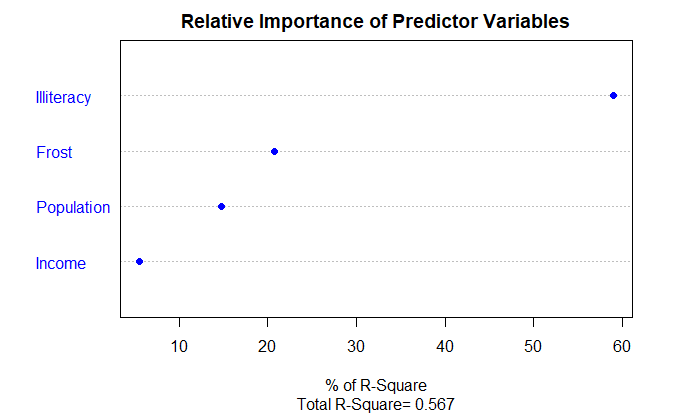
相对重要性
归一化
zstates <- as.data.frame(scale(states))
zfit <- lm(
  Murder ~ Population + Income + Illiteracy + Frost,
  data=zstates
)
coef(zfit)
  (Intercept)    Population        Income    Illiteracy         Frost
-2.054026e-16  2.705095e-01  1.072372e-02  6.840496e-01  8.185407e-03
相对权重,relative weight,对所有可能子模型添加一个预测变量引起的 R 平方平均增加量的一个近似值
relweights <- function(fit, ...) {
  R <- cor(fit$model)
  nvar <- ncol(R)

  rxx <- R[2:nvar, 2:nvar]
  rxy <- R[2:nvar, 1]

  svd <- eigen(rxx)
  evec <- svd$vectors
  ev <- svd$values
  delta <- diag(sqrt(ev))
  lambda <- evec %*% delta %*% t(evec)
  lambdasq <- lambda^2

  beta <- solve(lambda) %*% rxy
  rsquare <- colSums(beta ^ 2)
  rawwgt <- lambdasq %*% beta ^ 2

  import <- (rawwgt / rsquare) * 100
  import <- as.data.frame(import)
  row.names(import) <- names(fit$model[2:nvar])
  names(import) <- "Weights"
  import <- import[order(import), 1, drop=FALSE]
  dotchart(
    import$Weights,
    labels=row.names(import),
    xlab="% of R-Square",
    pch=19,
    main="Relative Importance of Predictor Variables",
    sub=paste("Total R-Square=", round(rsquare, digits=3)),
    ...
  )
  return(import)
}
fit <- lm(
  Murder ~ Population + Illiteracy + Income + Frost,
  data=states
)
relweights(fit, col="blue")
             Weights
Income      5.488962
Population 14.723401
Frost      20.787442
Illiteracy 59.000195
参考
https://github.com/perillaroc/r-in-action-study
R 语言实战
《图形初阶》
《基本数据管理》
《高级数据管理》
《基本图形》
《基本统计分析》
