R语言实战:图形初阶
目录
本文内容来自《R 语言实战》(R in Action, 2nd),有部分修改
使用图形
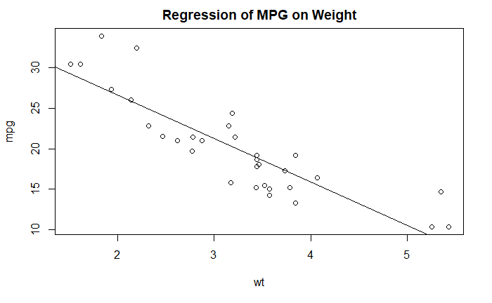
attach(mtcars)
plot(wt, mpg)
abline(lm(mpg ~ wt))
title("Regression of MPG on Weight")
detach(mtcars)
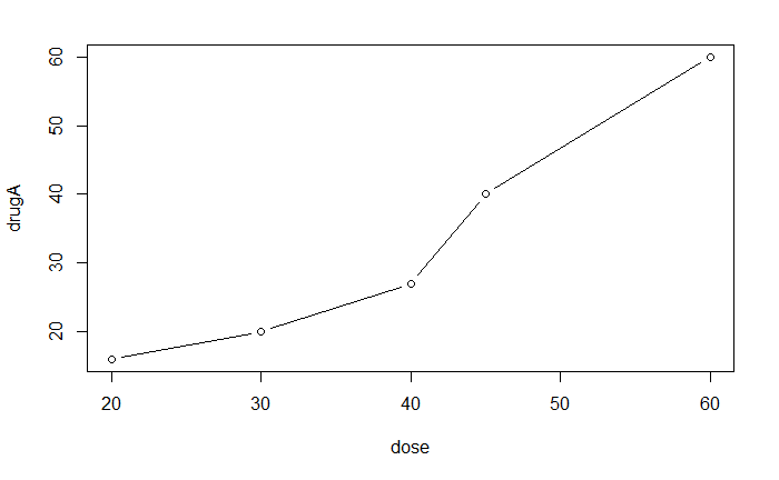
简单示例
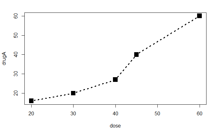
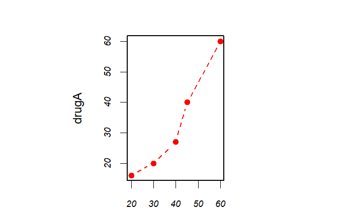
dose <- c(20, 30, 40, 45, 60)
drugA <- c(16, 20, 27, 40, 60)
drugB <- c(15, 18, 25, 31, 40)
plot(dose, drugA, type="b")
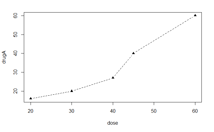
图形参数
使用 par() 函数设置绘图样式
opar <- par(no.readonly=TRUE)
par(lty=2, pch=17)
plot(dose, drugA, type="b")
par(opar)

某些参数可以直接在绘图函数中设置
plot(dose, drugA, type="b", lty=2, pch=17)
符号和线条
pch:点符号lty:线条类型cex:符号大小lwd:线条宽度
plot(
  dose, drugA,
  type="b",
  lty=3,
  lwd=3,
  pch=15,
  cex=2
)
颜色
col:默认颜色col.axiscol.labcol.maincol.sumfg:前景色bg:背景色
颜色值可以是:
- 序号
- 颜色名称
- 十六进制
- RGB
- HSV
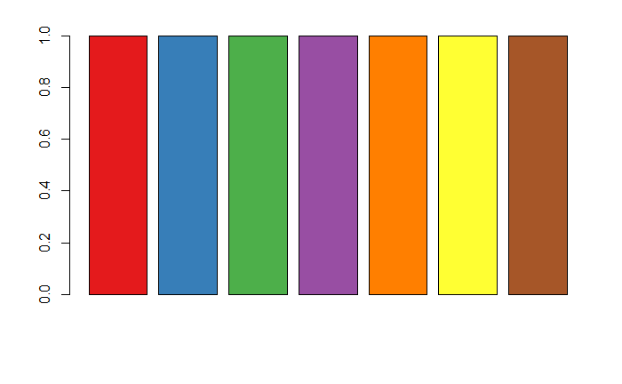
RColorBrewer 库
library(RColorBrewer)
n <- 7
mycolors <- brewer.pal(n, "Set1")
barplot(rep(1, n), col=mycolors)
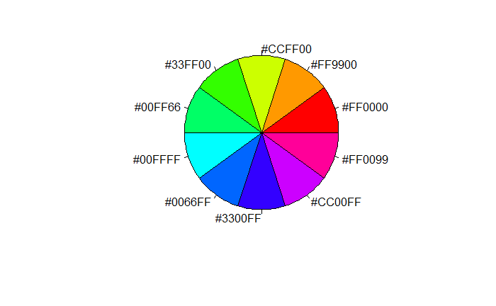
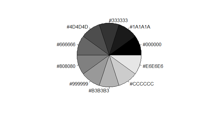
gray() 函数
n <- 10
mycolors <- rainbow(n)
pie(rep(1, n), labels=mycolors, col=mycolors)
mygrays <- gray(0:n/n)
pie(rep(1, n), labels=mygrays, col=mygrays)
文本属性
cex:大小font:字体ps:字体磅值family:字体族,标准取值为serif,sans,mono
图形尺寸与边界尺寸
pin:图形尺寸,英寸,宽和高mai:边界大小,英寸,下、左、上、右mar:边界大小,英分
opar <- par(no.readonly=TRUE)
par(pin=c(2, 3))
par(lwd=2, cex=1.5)
par(cex.axis=.75, font.axis=3)
plot(
dose, drugA,
type="b",
pch=19,
lty=2,
col="red"
)
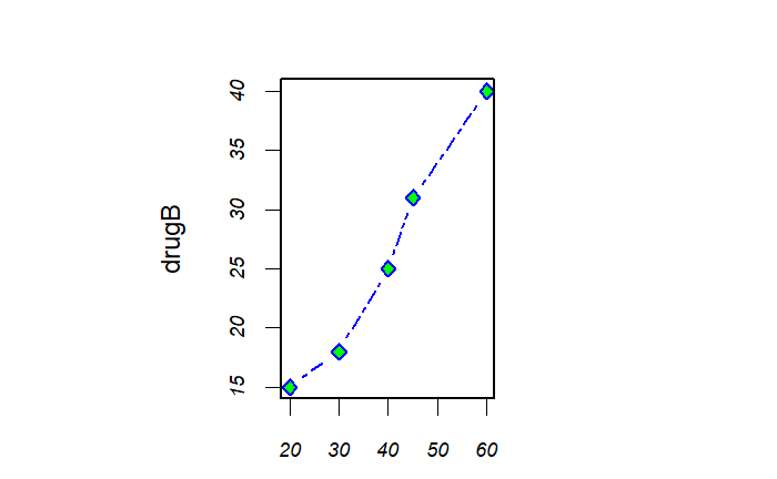
plot(
dose, drugB,
type="b",
pch=23,
lty=6,
col="blue",
bg="green"
)
par(opar)
添加文本、自定义坐标轴和图例
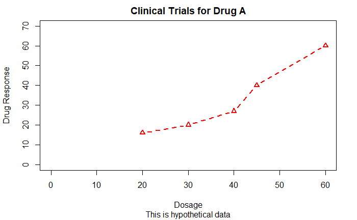
plot(
  dose, drugA,
  type="b",
  col="red",
  lty=2,
  pch=2,
  lwd=2,
  main="Clinical Trials for Drug A",
  sub="This is hypothetical data",
  xlab="Dosage",
  ylab="Drug Response",
  xlim=c(0, 60),
  ylim=c(0, 70)
)
标题
title()
坐标轴
axis()
side:坐标轴的位置,1 - 4at:刻度线位置labels:文字标签pos:轴线绘制位置,与另一坐标轴相交的位置ltycollas:标签平行(=0)或垂直(=1)于坐标轴tck:刻度线长度,正值内侧,负值外侧
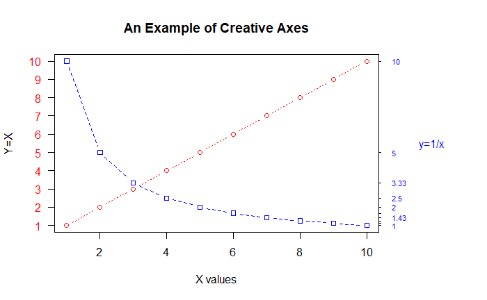
x <- 1:10
y <- x
z <- 10/x

opar <- par(no.readonly=TRUE)

par(mar=c(5, 4, 4, 8) + 0.1)
plot(
  x, y,
  type="b",
  pch=21,
  col="red",
  yaxt="n",
  lty=3,
  ann=FALSE
)
lines(
  x, z,
  type="b",
  pch=22,
  col="blue",
  lty=2
)

axis(
  2,
  at=x,
  labels=x,
  col.axis="red",
  las=2,
)

axis(
  4,
  at=z,
  labels=round(z, digits=2),
  col.axis="blue",
  las=2,
  cex.axis=0.7,
  tck=-.01
)

mtext(
  "y=1/x",
  side=4,
  line=3,
  cex.lab=1,
  las=2,
  col="blue"
)

title(
  "An Example of Creative Axes",
  xlab="X values",
  ylab="Y=X"
)

par(opar)
参考线
abline(h=yvalues, v=xvalues)
图例
legend()
locationtitlelegend:标签组成的字符型向量
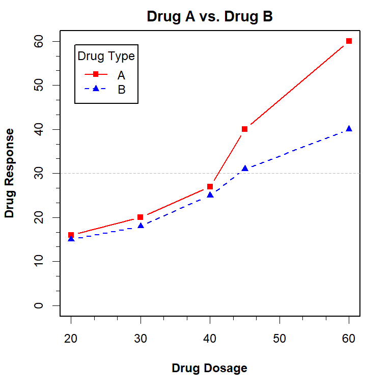
opar <- par(no.readonly=TRUE)

par(
  lwd=2,
  cex=1.5,
  font.lab=2
)

plot(
  dose, drugA,
  type="b",
  pch=15,
  lty=1,
  col="red",
  ylim=c(0, 60),
  main="Drug A vs. Drug B",
  xlab="Drug Dosage",
  ylab="Drug Response"
)

lines(
  dose, drugB,
  type="b",
  pch=17,
  lty=2,
  col="blue"
)

abline(
  h=c(30),
  lwd=1.5,
  lty=2,
  col="gray"
)

library(Hmisc)
minor.tick(
  nx=3,
  ny=3,
  tick.ratio=0.5
)

legend(
  "topleft",
  inset=.05,
  title="Drug Type",
  c("A", "B"),
  lty=c(1, 2),
  pch=c(15, 17),
  col=c("red", "blue")
)

par(opar)
文本标注
text()
mtext()
locationpos:1-4,文本相对于位置参数的方位side:1-4,放置文本的边
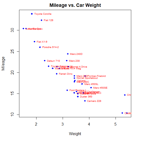
attach(mtcars)
plot(
  wt, mpg,
  main="Mileage vs. Car Weight",
  xlab="Weight",
  ylab="Mileage",
  pch=18,
  col="blue"
)

text(
  wt, mpg,
  row.names(mtcars),
  cex=0.6,
  pos=4,
  col="red"
)
detach(mtcars)
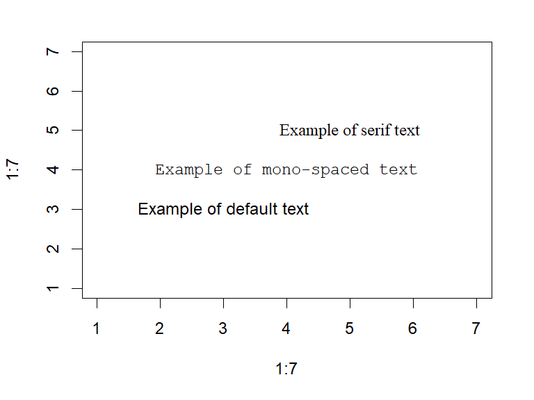
opar <- par(no.readonly=TRUE)
par(cex=1.5)

plot(
  1:7, 1:7,
  type="n"
)

text(
  3, 3,
  "Example of default text"
)
text(
  4, 4,
  family="mono",
  "Example of mono-spaced text"
)
text(
  5, 5,
  family="serif",
  "Example of serif text"
)

par(opar)
数学标注
plotmath
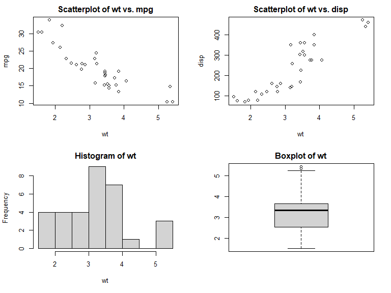
图形的组合
par() 函数的 mfrow=c(nrows, ncols)
layout()
两行两列
attach(mtcars)
opar <- par(no.readonly=TRUE)
par(mfrow=c(2, 2))

plot(
  wt, mpg,
  main="Scatterplot of wt vs. mpg"
)
plot(
  wt, disp,
  main="Scatterplot of wt vs. disp"
)
hist(
  wt,
  main="Histogram of wt"
)
boxplot(
  wt,
  main="Boxplot of wt"
)

par(opar)
detach(mtcars)
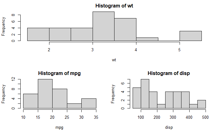
三行一列
attach(mtcars)
opar <- par(no.readonly=TRUE)
par(mfrow=c(3, 1))
hist(wt)
hist(mpg)
hist(disp)
par(opar)
detach(mtcars)
layout()
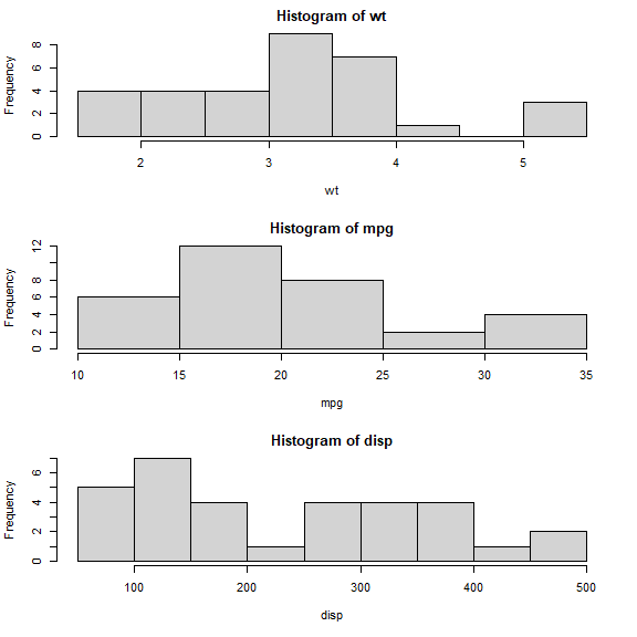
attach(mtcars)
layout(
  matrix(
    c(1, 1, 2, 3),
    2, 2,
    byrow=TRUE
  )
)
hist(wt)
hist(mpg)
hist(disp)
detach(mtcars)
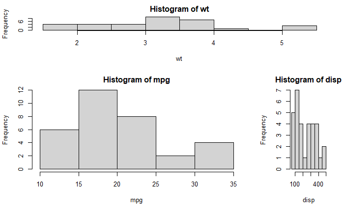
widths 和 heights 参数
attach(mtcars)
layout(
  matrix(
    c(1, 1, 2, 3),
    2, 2,
    byrow=TRUE
  ),
  widths=c(3, 1),
  heights=c(1, 2)
)
hist(wt)
hist(mpg)
hist(disp)
detach(mtcars)
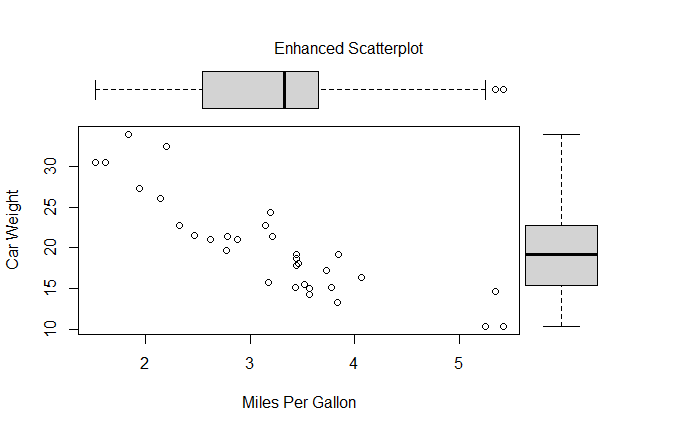
布局的精细控制:fig 参数
opar <- par(no.readonly=TRUE)
par(fig=c(0, 0.8, 0, 0.8))
plot(
  mtcars$wt, mtcars$mpg,
  xlab="Miles Per Gallon",
  ylab="Car Weight"
)

par(fig=c(0, 0.8, 0.45, 1), new=TRUE)
boxplot(
  mtcars$wt,
  horizontal=TRUE,
  axes=FALSE
)

par(
  fig=c(0.55, 1, 0, 0.8),
  new=TRUE
)
boxplot(mtcars$mpg, axes=FALSE)

mtext(
  "Enhanced Scatterplot",
  side=3,
  outer=TRUE,
  line=-3
)

par(opar)