ISLR实验:分类 - 线性判别分析
目录
本文源自《统计学习导论:基于R语言应用》(ISLR) 中《4.6 R实验:逻辑斯谛回归、LDA、QDA和KNN》章节
library(ISLR)
library(MASS)
library(pROC)
数据
股票市场数据
data(Smarket)
head(Smarket)
  Year   Lag1   Lag2   Lag3   Lag4   Lag5 Volume  Today Direction
1 2001  0.381 -0.192 -2.624 -1.055  5.010 1.1913  0.959        Up
2 2001  0.959  0.381 -0.192 -2.624 -1.055 1.2965  1.032        Up
3 2001  1.032  0.959  0.381 -0.192 -2.624 1.4112 -0.623      Down
4 2001 -0.623  1.032  0.959  0.381 -0.192 1.2760  0.614        Up
5 2001  0.614 -0.623  1.032  0.959  0.381 1.2057  0.213        Up
6 2001  0.213  0.614 -0.623  1.032  0.959 1.3491  1.392        Up
训练集和测试集
训练集:2001 至 2004 年
测试集:2005 年
train <- (Year < 2005)
train 是一个布尔变量,Boolean vector
smarket_2005 <- Smarket[!train, ]
dim(smarket_2005)
[1] 252 9
direction_2005 <- Direction[!train]
方法
MASS 包的 lda() 函数实现线性判别分析
lda_fit <- lda(
  Direction ~ Lag1 + Lag2,
  data=Smarket,
  subset=train
)
lda_fit
Call:
lda(Direction ~ Lag1 + Lag2, data = Smarket, subset = train)

Prior probabilities of groups:
    Down       Up
0.491984 0.508016

Group means:
            Lag1        Lag2
Down  0.04279022  0.03389409
Up   -0.03954635 -0.03132544

Coefficients of linear discriminants:
            LD1
Lag1 -0.6420190
Lag2 -0.5135293
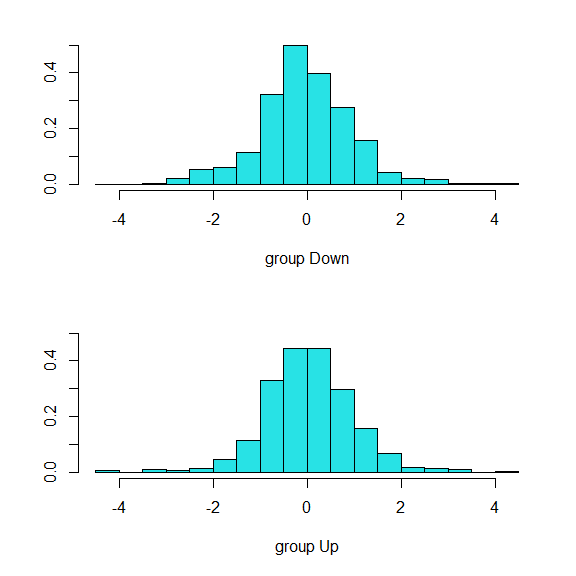
plot() 函数生成线性判别图像
plot(lda_fit)
预测
predict() 返回三元列表
- class 存储预测结果
- posterior 是后验概率
- x 是线性判别
lda_predict <- predict(
  lda_fit,
  smarket_2005
)
names(lda_predict)
[1] "class" "posterior" "x"
后验概率
lda_predict$posterior[1:20, ]
          Down        Up
999  0.4901792 0.5098208
1000 0.4792185 0.5207815
1001 0.4668185 0.5331815
1002 0.4740011 0.5259989
1003 0.4927877 0.5072123
1004 0.4938562 0.5061438
1005 0.4951016 0.5048984
1006 0.4872861 0.5127139
1007 0.4907013 0.5092987
1008 0.4844026 0.5155974
1009 0.4906963 0.5093037
1010 0.5119988 0.4880012
1011 0.4895152 0.5104848
1012 0.4706761 0.5293239
1013 0.4744593 0.5255407
1014 0.4799583 0.5200417
1015 0.4935775 0.5064225
1016 0.5030894 0.4969106
1017 0.4978806 0.5021194
1018 0.4886331 0.5113669
预测结果
lda_predict$class[1:20]
 [1] Up   Up   Up   Up   Up   Up   Up   Up   Up   Up   Up   Down Up
[14] Up   Up   Up   Up   Down Up   Up
Levels: Down Up
线性判据
lda_predict$x[1:20]
 [1]  0.08293096  0.59114102  1.16723063  0.83335022 -0.03792892
 [6] -0.08743142 -0.14512719  0.21701324  0.05873792  0.35068642
[11]  0.05897298 -0.92794134  0.11370190  0.98783874  0.81206862
[16]  0.55681363 -0.07452314 -0.51514029 -0.27386231  0.15458312
列联表
lda_class <- lda_predict$class
table(direction_2005, lda_class)
              lda_class
direction_2005 Down  Up
          Down   35  76
          Up     35 106
mean(lda_class == direction_2005)
[1] 0.5595238
class 使用 50% 作为阈值
sum(lda_predict$posterior[,1] > .5)
[1] 70
sum(lda_predict$posterior[,1] <= .5)
[1] 182
使用 90% 作为阈值
sum(lda_predict$posterior[,1] > .9)
[1] 0
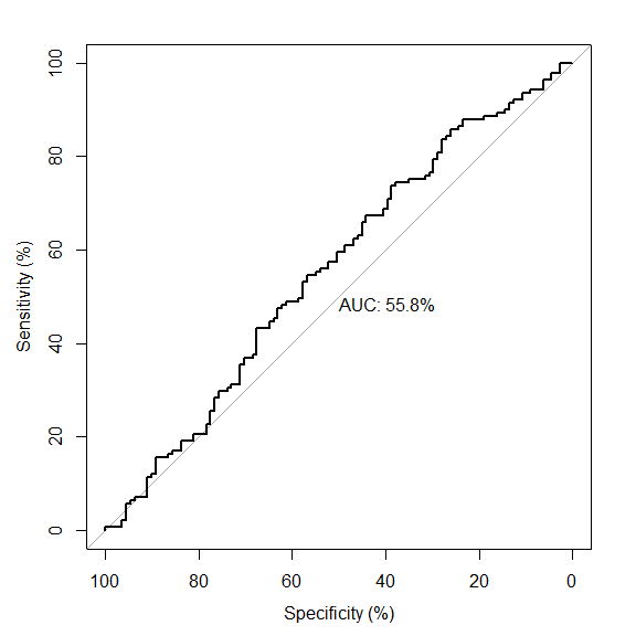
ROC 曲线
plot(
  roc(
    direction_2005,
    lda_predict$posterior[,2],
    percent=TRUE
  ),
  print.auc=TRUE,
  plot=TRUE
)
参考
https://github.com/perillaroc/islr-study
ISLR实验系列文章
线性回归
分类
重抽样方法
线性模型选择与正则化
