ISLR实验:线性模型扩展
本文源自《统计学习导论:基于R语言应用》(ISLR) 中《3.6 实验:线性回归》章节
标准线性回归模型有两个最重要的假设:
- 可加性 (additive):预测变量 X_j 的变化对响应变量 Y 产生的影响与其他预测变量的取值无关。
- 线性 (linear):无论 X_j 取何值,X_j 变化一个单位引起的响应变量 Y 的变化是恒定的。
上述假设在实际问题中常常被违背。
本文介绍一些扩展的线性模型,继续使用 Boston 数据集。
library(MASS)
library(ISLR)
交互项
交互项 (interaction) 去除可加性假设,考虑变量之间的交互作用 (interaction)。
使用两个变量的乘积作为一个交互项。
lm() 支持交互项。
lstat:black 将 lstat 和 black 的交互项加入到模型中。
lstat*age 将 lstat,age 和交互项 lstat * age 作为预测变量,是 lstat + age + lstat:age 的简写
lm.fit.inter <- lm(medv~lstat * age, data=Boston)
lm.fit.inter
Call:
lm(formula = medv ~ lstat * age, data = Boston)

Coefficients:
(Intercept)        lstat          age    lstat:age
 36.0885359   -1.3921168   -0.0007209    0.0041560
summary(lm.fit.inter)
Call:
lm(formula = medv ~ lstat * age, data = Boston)

Residuals:
    Min      1Q  Median      3Q     Max
-15.806  -4.045  -1.333   2.085  27.552

Coefficients:
              Estimate Std. Error t value Pr(>|t|)
(Intercept) 36.0885359  1.4698355  24.553  < 2e-16 ***
lstat       -1.3921168  0.1674555  -8.313 8.78e-16 ***
age         -0.0007209  0.0198792  -0.036   0.9711
lstat:age    0.0041560  0.0018518   2.244   0.0252 *
---
Signif. codes:  0 ‘***’ 0.001 ‘**’ 0.01 ‘*’ 0.05 ‘.’ 0.1 ‘ ’ 1

Residual standard error: 6.149 on 502 degrees of freedom
Multiple R-squared:  0.5557,	Adjusted R-squared:  0.5531
F-statistic: 209.3 on 3 and 502 DF,  p-value: < 2.2e-16
实验分层原则 (hierarchical principle) 规定:
如果模型中含有交互项,那么即使主效应的系数的 p 值不显著,也应包含在模型中。
虽然上述模型中 age 的 p 值较大,但 age 也应该包含在模型中。
预测变量的非线性变换
一种简单的非线性关系就是 多项式回归 (polynomial regression)。
lm() 函数支持预测变量的非线性变换。
对于预测变量 X,可以使用 I(X^2) 创建预测变量 X^2。
建立 medv 对 lstat 和 lstat^2 的回归
lm.fit.power <- lm(medv~lstat + I(lstat^2), data=Boston)
lm.fit.power
Call:
lm(formula = medv ~ lstat + I(lstat^2), data = Boston)

Coefficients:
(Intercept)        lstat   I(lstat^2)
   42.86201     -2.33282      0.04355
summary(lm.fit.power)
Call:
lm(formula = medv ~ lstat + I(lstat^2), data = Boston)

Residuals:
     Min       1Q   Median       3Q      Max
-15.2834  -3.8313  -0.5295   2.3095  25.4148

Coefficients:
             Estimate Std. Error t value Pr(>|t|)
(Intercept) 42.862007   0.872084   49.15   <2e-16 ***
lstat       -2.332821   0.123803  -18.84   <2e-16 ***
I(lstat^2)   0.043547   0.003745   11.63   <2e-16 ***
---
Signif. codes:  0 ‘***’ 0.001 ‘**’ 0.01 ‘*’ 0.05 ‘.’ 0.1 ‘ ’ 1

Residual standard error: 5.524 on 503 degrees of freedom
Multiple R-squared:  0.6407,	Adjusted R-squared:  0.6393
F-statistic: 448.5 on 2 and 503 DF,  p-value: < 2.2e-16
二次项的 p 值接近零,表示它使模型得到改进。
验证
使用 anova() 函数量化二次拟合在何种程度上优于线性组合。
lm.fit <- lm(medv~lstat, data=Boston)
summary(lm.fit)
Call:
lm(formula = medv ~ lstat, data = Boston)

Residuals:
    Min      1Q  Median      3Q     Max
-15.168  -3.990  -1.318   2.034  24.500

Coefficients:
            Estimate Std. Error t value Pr(>|t|)
(Intercept) 34.55384    0.56263   61.41   <2e-16 ***
lstat       -0.95005    0.03873  -24.53   <2e-16 ***
---
Signif. codes:  0 ‘***’ 0.001 ‘**’ 0.01 ‘*’ 0.05 ‘.’ 0.1 ‘ ’ 1

Residual standard error: 6.216 on 504 degrees of freedom
Multiple R-squared:  0.5441,	Adjusted R-squared:  0.5432
F-statistic: 601.6 on 1 and 504 DF,  p-value: < 2.2e-16
anova(lm.fit, lm.fit.power)
Analysis of Variance Table

Model 1: medv ~ lstat
Model 2: medv ~ lstat + I(lstat^2)
  Res.Df   RSS Df Sum of Sq     F    Pr(>F)
1    504 19472
2    503 15347  1    4125.1 135.2 < 2.2e-16 ***
---
Signif. codes:  0 ‘***’ 0.001 ‘**’ 0.01 ‘*’ 0.05 ‘.’ 0.1 ‘ ’ 1
模型 1 是线性模型,模型 2 是包含一次项和二次项的二次模型
anova() 通过假设检验比较两个模型。
- 零假设:这两个模型拟合效果相当
- 备择假设:二次模型效果更优
上述结果中,F 统计量为 135,p 值几乎为 0,表明二次模型远远优于一次模型。
绘图
par(mfrow=c(2, 2))
plot(lm.fit.power)
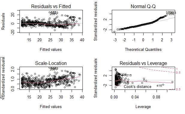
残差中可识别的规律很少
多项式拟合
使用 poly() 和 lm() 可以创建多项式拟合
5 阶多项式拟合
lm.fit.5 <- lm(medv~poly(lstat, 5), data=Boston)
summary(lm.fit.5)
Call:
lm(formula = medv ~ poly(lstat, 5), data = Boston)

Residuals:
     Min       1Q   Median       3Q      Max
-13.5433  -3.1039  -0.7052   2.0844  27.1153

Coefficients:
                 Estimate Std. Error t value Pr(>|t|)
(Intercept)       22.5328     0.2318  97.197  < 2e-16 ***
poly(lstat, 5)1 -152.4595     5.2148 -29.236  < 2e-16 ***
poly(lstat, 5)2   64.2272     5.2148  12.316  < 2e-16 ***
poly(lstat, 5)3  -27.0511     5.2148  -5.187 3.10e-07 ***
poly(lstat, 5)4   25.4517     5.2148   4.881 1.42e-06 ***
poly(lstat, 5)5  -19.2524     5.2148  -3.692 0.000247 ***
---
Signif. codes:  0 ‘***’ 0.001 ‘**’ 0.01 ‘*’ 0.05 ‘.’ 0.1 ‘ ’ 1

Residual standard error: 5.215 on 500 degrees of freedom
Multiple R-squared:  0.6817,	Adjusted R-squared:  0.6785
F-statistic: 214.2 on 5 and 500 DF,  p-value: < 2.2e-16
上述结果表明,5 阶以下的多项式改善了模型的效果。
更高阶模型
lm.fit.8 <- lm(medv~poly(lstat, 8), data=Boston)
summary(lm.fit.8)
Call:
lm(formula = medv ~ poly(lstat, 8), data = Boston)

Residuals:
     Min       1Q   Median       3Q      Max
-13.7394  -3.1475  -0.7329   2.0959  26.9915

Coefficients:
                 Estimate Std. Error t value Pr(>|t|)
(Intercept)       22.5328     0.2317  97.233  < 2e-16 ***
poly(lstat, 8)1 -152.4595     5.2129 -29.247  < 2e-16 ***
poly(lstat, 8)2   64.2272     5.2129  12.321  < 2e-16 ***
poly(lstat, 8)3  -27.0511     5.2129  -5.189 3.08e-07 ***
poly(lstat, 8)4   25.4517     5.2129   4.882 1.41e-06 ***
poly(lstat, 8)5  -19.2524     5.2129  -3.693 0.000246 ***
poly(lstat, 8)6    6.5088     5.2129   1.249 0.212404
poly(lstat, 8)7    1.9416     5.2129   0.372 0.709703
poly(lstat, 8)8   -6.7299     5.2129  -1.291 0.197302
---
Signif. codes:  0 ‘***’ 0.001 ‘**’ 0.01 ‘*’ 0.05 ‘.’ 0.1 ‘ ’ 1

Residual standard error: 5.213 on 497 degrees of freedom
Multiple R-squared:  0.6838,	Adjusted R-squared:  0.6787
F-statistic: 134.4 on 8 and 497 DF,  p-value: < 2.2e-16
5 阶以上的多项式的 p 值不显著
对数变换
lm() 也支持其他种类的非线性变换,比如对数变换
lm.fit.log <- lm(medv~log(rm), data=Boston)
summary(lm.fit.log)
Call:
lm(formula = medv ~ log(rm), data = Boston)

Residuals:
    Min      1Q  Median      3Q     Max
-19.487  -2.875  -0.104   2.837  39.816

Coefficients:
            Estimate Std. Error t value Pr(>|t|)
(Intercept)  -76.488      5.028  -15.21   <2e-16 ***
log(rm)       54.055      2.739   19.73   <2e-16 ***
---
Signif. codes:  0 ‘***’ 0.001 ‘**’ 0.01 ‘*’ 0.05 ‘.’ 0.1 ‘ ’ 1

Residual standard error: 6.915 on 504 degrees of freedom
Multiple R-squared:  0.4358,	Adjusted R-squared:  0.4347
F-statistic: 389.3 on 1 and 504 DF,  p-value: < 2.2e-16
定性预测变量
研究 Carseats 数据集(汽车座椅)。
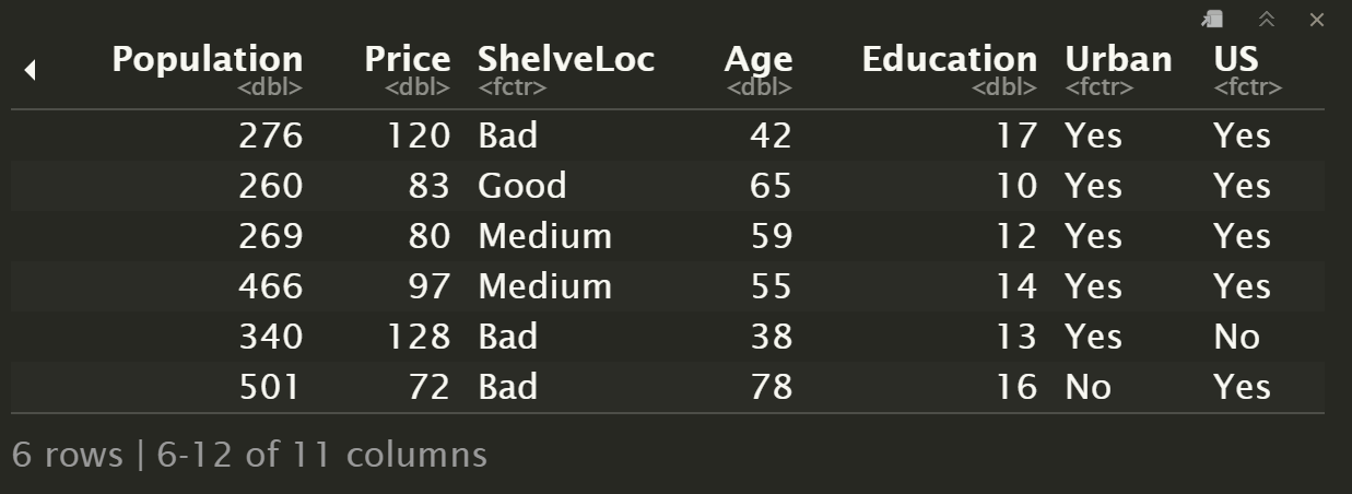
head(Carseats)
names(Carseats)
 [1] "Sales"       "CompPrice"   "Income"      "Advertising" "Population"  "Price"
 [7] "ShelveLoc"   "Age"         "Education"   "Urban"       "US"
ShelveLoc 是定性变量,也称为 因子 (factor),表示每个地区搁架位置的质量指标,即在每个地区汽车座椅在商店内的展示空间。 有三个可能的取值,称为 水平 (levels):
- 坏:
Bad - 中等:
Medium - 好:
good
数据集中已指定 ShelveLoc 为 factor 类型,R 将自动生成虚拟变量。
构建一个包含交互项的多元回归模型
lm.fit.factor <- lm(
  Sales~.+Income:Advertising + Price:Age,
  data=Carseats
)
summary(lm.fit.factor)
Call:
lm(formula = Sales ~ . + Income:Advertising + Price:Age, data = Carseats)

Residuals:
    Min      1Q  Median      3Q     Max
-2.9208 -0.7503  0.0177  0.6754  3.3413

Coefficients:
                     Estimate Std. Error t value Pr(>|t|)
(Intercept)         6.5755654  1.0087470   6.519 2.22e-10 ***
CompPrice           0.0929371  0.0041183  22.567  < 2e-16 ***
Income              0.0108940  0.0026044   4.183 3.57e-05 ***
Advertising         0.0702462  0.0226091   3.107 0.002030 **
Population          0.0001592  0.0003679   0.433 0.665330
Price              -0.1008064  0.0074399 -13.549  < 2e-16 ***
ShelveLocGood       4.8486762  0.1528378  31.724  < 2e-16 ***
ShelveLocMedium     1.9532620  0.1257682  15.531  < 2e-16 ***
Age                -0.0579466  0.0159506  -3.633 0.000318 ***
Education          -0.0208525  0.0196131  -1.063 0.288361
UrbanYes            0.1401597  0.1124019   1.247 0.213171
USYes              -0.1575571  0.1489234  -1.058 0.290729
Income:Advertising  0.0007510  0.0002784   2.698 0.007290 **
Price:Age           0.0001068  0.0001333   0.801 0.423812
---
Signif. codes:  0 ‘***’ 0.001 ‘**’ 0.01 ‘*’ 0.05 ‘.’ 0.1 ‘ ’ 1

Residual standard error: 1.011 on 386 degrees of freedom
Multiple R-squared:  0.8761,	Adjusted R-squared:  0.8719
F-statistic:   210 on 13 and 386 DF,  p-value: < 2.2e-16
constrasts() 函数返回 R 虚拟变量的编码
contrasts(Carseats$ShelveLoc)

R 创建两个 哑变量 (dummy variable):
ShelveLocGood:值为 1 时表示 GoodShelveLocMedium:值为 1 是表示 Medium
两个变量值均为 0 时,表示 Bad
注意:这两个变量不能同时为 1
回归模型中,ShelveLocGood 系数为正,表明好的货架位置与高销售额相关。
ShelveLocMedium 系数为较小的正值,表明中等水平货架位置的销量比坏位置高,但比一个好位置差。
参考
https://github.com/perillaroc/islr-study
ISLR实验系列文章
线性回归
分类
重抽样方法
线性模型选择与正则化
