xarray指南:插值
本文翻译自 xarray 官方文档 Interpolating data 的部分内容。
首先导入需要使用到的库。
import numpy as np
import pandas as pd
import xarray as xr
import matplotlib.pyplot as plt
xarray 提供了灵活的插值程序,与索引有相似的接口。
注意:interp 需要安装 scipy
标量和一维插值
插值 DataArray 和标签索引 DataArray 的工作方式类似。
da = xr.DataArray(
    np.sin(0.3 * np.arange(12).reshape(4, 3)),
    [
        ("time", np.arange(4)),
        ("space", [0.1, 0.2, 0.3]),
    ]
)
da
<xarray.DataArray (time: 4, space: 3)>
array([[ 0.        ,  0.29552021,  0.56464247],
       [ 0.78332691,  0.93203909,  0.99749499],
       [ 0.97384763,  0.86320937,  0.67546318],
       [ 0.42737988,  0.14112001, -0.15774569]])
Coordinates:
  * time     (time) int64 0 1 2 3
  * space    (space) float64 0.1 0.2 0.3
标签查找
da.sel(time=3)
<xarray.DataArray (space: 3)>
array([ 0.42737988,  0.14112001, -0.15774569])
Coordinates:
    time     int64 3
  * space    (space) float64 0.1 0.2 0.3
插值
da.interp(time=2.5)
<xarray.DataArray (space: 3)>
array([0.70061376, 0.50216469, 0.25885874])
Coordinates:
  * space    (space) float64 0.1 0.2 0.3
    time     float64 2.5
注意:未设置 method 参数的标签查找仅支持已存在的坐标值。
与索引类似,interp 也接受数组形式的参数,返回数组形式的插值结果
标签查找
da.sel(time=[2, 3])
<xarray.DataArray (time: 2, space: 3)>
array([[ 0.97384763,  0.86320937,  0.67546318],
       [ 0.42737988,  0.14112001, -0.15774569]])
Coordinates:
  * time     (time) int64 2 3
  * space    (space) float64 0.1 0.2 0.3
插值
da.interp(time=[2.5, 3.5])
<xarray.DataArray (time: 2, space: 3)>
array([[0.70061376, 0.50216469, 0.25885874],
       [       nan,        nan,        nan]])
Coordinates:
  * space    (space) float64 0.1 0.2 0.3
  * time     (time) float64 2.5 3.5
对带有 numpy.datetime64 坐标的数据插值,可以传递字符串
da_dt64 = xr.DataArray(
    [1, 3],
    [
        ("time", pd.date_range("1/1/2000", "1/3/2000", periods=2))
    ]
)
da_dt64
<xarray.DataArray (time: 2)>
array([1, 3])
Coordinates:
  * time     (time) datetime64[ns] 2000-01-01 2000-01-03
da_dt64.interp(
    time="2000-01-02"
)
<xarray.DataArray ()>
array(2.)
Coordinates:
    time     datetime64[ns] 2000-01-02
通过指定所需的时间段,可以将插值后的数据合并到原始 DataArray 中。
da_dt64.interp(
    time=pd.date_range(
        "1/1/2000",
        "1/3/2000",
        periods=3
    )
)
<xarray.DataArray (time: 3)>
array([1., 2., 3.])
Coordinates:
  * time     (time) datetime64[ns] 2000-01-01 2000-01-02 2000-01-03
也可以对使用 CFTimeIndex 索引的数据进行插值。
注意
当前,我们的插值仅适用于常规网格。
因此,与 sel() 类似,只有沿维度的一维坐标才可以用于插值的原始坐标。
多维插值
与 sel() 类似,interp() 接收多个坐标。
这种情况下,将进行多维插值。
标签查找
da.sel(
    time=2,
    space=0.1,
)
<xarray.DataArray ()>
array(0.97384763)
Coordinates:
    time     int64 2
    space    float64 0.1
插值
da.interp(
    time=2.5,
    space=0.15
)
<xarray.DataArray ()>
array(0.60138922)
Coordinates:
    time     float64 2.5
    space    float64 0.15
同样接收数组形式的参数
标签查找
da.sel(
    time=[2, 3],
    space=[0.1, 0.2]
)
<xarray.DataArray (time: 2, space: 2)>
array([[0.97384763, 0.86320937],
       [0.42737988, 0.14112001]])
Coordinates:
  * time     (time) int64 2 3
  * space    (space) float64 0.1 0.2
插值
da.interp(
    time=[1.5, 2.5],
    space=[0.15, 0.25],
)
<xarray.DataArray (time: 2, space: 2)>
array([[0.88810575, 0.86705165],
       [0.60138922, 0.38051172]])
Coordinates:
  * time     (time) float64 1.5 2.5
  * space    (space) float64 0.15 0.25
interp_like() 方法是一个有用的快捷方式。
此方法将 xarray 对象插值到另一个 xarray 对象的坐标上。
例如,如果我们想要计算两个坐标略有不同的 DataArray (da 和 other)之间的差异。
other = xr.DataArray(
    np.sin(0.4 * np.arange(9).reshape(3, 3)),
    [
        ("time", [0.9, 1.9, 2.9]),
        ("space", [0.15, 0.25, 0.35]),
    ]
)
other
<xarray.DataArray (time: 3, space: 3)>
array([[ 0.        ,  0.38941834,  0.71735609],
       [ 0.93203909,  0.9995736 ,  0.90929743],
       [ 0.67546318,  0.33498815, -0.05837414]])
Coordinates:
  * time     (time) float64 0.9 1.9 2.9
  * space    (space) float64 0.15 0.25 0.35
最好先对 da 进行插值,使其保持在 other 坐标上,然后再减去它。
interp_like() 可用于这种情况。
# 沿 oeter 的坐标插值 da
interpolated = da.interp_like(other)
interpolated
<xarray.DataArray (time: 3, space: 3)>
array([[0.78669071, 0.91129847,        nan],
       [0.91244395, 0.78887935,        nan],
       [0.3476778 , 0.06945207,        nan]])
Coordinates:
  * time     (time) float64 0.9 1.9 2.9
  * space    (space) float64 0.15 0.25 0.35
现在可以安全地计算 other - interpolated 差异了。
other - interpolated
<xarray.DataArray (time: 3, space: 3)>
array([[-0.78669071, -0.52188012,         nan],
       [ 0.01959514,  0.21069425,         nan],
       [ 0.32778538,  0.26553608,         nan]])
Coordinates:
  * time     (time) float64 0.9 1.9 2.9
  * space    (space) float64 0.15 0.25 0.35
插值方法
我们使用 scipy.interpolate.interp1d 对一维数据插值,使用 scipy.interpolate.interpn() 对多维数据插值。
可以通过可选的 method 参数指定插值方法。
da = xr.DataArray(
    np.sin(np.linspace(0, 2 * np.pi, 10)),
    dims="x",
    coords={
        "x": np.linspace(0, 1, 10),
    }
)
da
<xarray.DataArray (x: 10)>
array([ 0.00000000e+00,  6.42787610e-01,  9.84807753e-01,  8.66025404e-01,
        3.42020143e-01, -3.42020143e-01, -8.66025404e-01, -9.84807753e-01,
       -6.42787610e-01, -2.44929360e-16])
Coordinates:
  * x        (x) float64 0.0 0.1111 0.2222 0.3333 ... 0.6667 0.7778 0.8889 1.0
da.plot.line('o', label="original")

da.interp(
    x=np.linspace(0, 1, 100)
).plot.line(
    label='linear (default)'
)

da.interp(
    x=np.linspace(0, 1, 100),
    method='cubic'
).plot.line(
    label='cubic'
)

plt.legend()
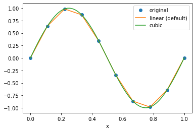
附加的关键词参数 kwargs 会传递给 scipy 函数。
原始坐标范围外的点填充 0
da.interp(
    x=np.linspace(-0.5, 1.5, 10),
    kwargs={
        'fill_value': 0.0
    }
)
<xarray.DataArray (x: 10)>
array([ 0.        ,  0.        ,  0.        ,  0.81379768,  0.60402277,
       -0.60402277, -0.81379768,  0.        ,  0.        ,  0.        ])
Coordinates:
  * x        (x) float64 -0.5 -0.2778 -0.05556 0.1667 ... 0.8333 1.056 1.278 1.5
外推
da.interp(
    x=np.linspace(-0.5, 1.5, 10),
    kwargs={
        'fill_value': 'extrapolate'
    }
)
<xarray.DataArray (x: 10)>
array([-2.89254424, -1.60696902, -0.3213938 ,  0.81379768,  0.60402277,
       -0.60402277, -0.81379768,  0.3213938 ,  1.60696902,  2.89254424])
Coordinates:
  * x        (x) float64 -0.5 -0.2778 -0.05556 0.1667 ... 0.8333 1.056 1.278 1.5
高级插值
interp() 与 sel() 类似,接收 DataArray,提供更高级的插值。
根据传递给 interp() 的新坐标维度,确定返回结果的维度。
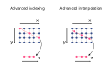
例如,如果要沿特定维度插值二维数组,如下图所示,则可以传递两个具有共同维度的一维 DataArray 作为新坐标。
例如:
da = xr.DataArray(
    np.sin(0.3 * np.arange(20).reshape(5, 4)),
    [
        ('x', np.arange(5)),
        ('y', [0.1, 0.2, 0.3, 0.4])
    ]
)
da
<xarray.DataArray (x: 5, y: 4)>
array([[ 0.        ,  0.29552021,  0.56464247,  0.78332691],
       [ 0.93203909,  0.99749499,  0.97384763,  0.86320937],
       [ 0.67546318,  0.42737988,  0.14112001, -0.15774569],
       [-0.44252044, -0.68776616, -0.87157577, -0.97753012],
       [-0.99616461, -0.92581468, -0.77276449, -0.55068554]])
Coordinates:
  * x        (x) int64 0 1 2 3 4
  * y        (y) float64 0.1 0.2 0.3 0.4
高级索引
x = xr.DataArray([0, 2, 4], dims='z')
y = xr.DataArray([0.1, 0.2, 0.3], dims='z')

da.sel(x=x, y=y)
<xarray.DataArray (z: 3)>
array([ 0.        ,  0.42737988, -0.77276449])
Coordinates:
    x        (z) int64 0 2 4
    y        (z) float64 0.1 0.2 0.3
Dimensions without coordinates: z
高级插值
x = xr.DataArray([0.5, 1.5, 2.5], dims='z')
y = xr.DataArray([0.15, 0.25, 0.35], dims='z')
da.interp(x=x, y=y)
<xarray.DataArray (z: 3)>
array([ 0.55626357,  0.63496063, -0.46643289])
Coordinates:
    x        (z) float64 0.5 1.5 2.5
    y        (z) float64 0.15 0.25 0.35
Dimensions without coordinates: z
原始坐标 (x, y) = ((0.5, 0.15), (1.5, 0.25), (2.5, 0.35)) 的值通过二维插值获得,并映射到新的维度 z。
如果想要为新的维度 z 添加坐标,可以为 DataArray 提供坐标。
x = xr.DataArray(
    [0.5, 1.5, 2.5],
    dims='z',
    coords={
        'z': ['a', 'b','c']
    }
)

y = xr.DataArray(
    [0.15, 0.25, 0.35],
    dims='z',
    coords={
        'z': ['a', 'b','c']
    }
)

da.interp(x=x, y=y)
<xarray.DataArray (z: 3)>
array([ 0.55626357,  0.63496063, -0.46643289])
Coordinates:
    x        (z) float64 0.5 1.5 2.5
    y        (z) float64 0.15 0.25 0.35
  * z        (z) <U1 'a' 'b' 'c'
插值带 NaN 值的数组
我们的 interp() 处理带 NaN 值的数组时使用与 scipy.interpolate.interp1d 和 scipy.interpolate.interpn 一样的方法。linear 和 nearest 方法返回包含 NaN 的数组,而其他方法返回所有值都为 NaN 的数组,例如 cubic 和 quadratic。
da = xr.DataArray(
    [0, 2, np.nan, 3, 3.25],
    dims="x",
    coords={"x": range(5)}
)
da
<xarray.DataArray (x: 5)>
array([0.  , 2.  ,  nan, 3.  , 3.25])
Coordinates:
  * x        (x) int64 0 1 2 3 4
da.interp(
    x=[0.5, 1.5, 2.5]
)
<xarray.DataArray (x: 3)>
array([ 1., nan, nan])
Coordinates:
  * x        (x) float64 0.5 1.5 2.5
da.interp(
    x=[0.5, 1.5, 2.5],
    method="cubic",
)
<xarray.DataArray (x: 3)>
array([nan, nan, nan])
Coordinates:
  * x        (x) float64 0.5 1.5 2.5
为了避免这种情况,您可以通过 dropna() 删除 NaN,然后进行插值
dropped = da.dropna("x")
dropped
<xarray.DataArray (x: 4)>
array([0.  , 2.  , 3.  , 3.25])
Coordinates:
  * x        (x) int64 0 1 3 4
dropped.interp(
    x=[0.5, 1.5, 2.5],
    method="cubic"
)
<xarray.DataArray (x: 3)>
array([1.19010417, 2.5078125 , 2.9296875 ])
Coordinates:
  * x        (x) float64 0.5 1.5 2.5
如果 NaN 在多维数组中随机分布,使用 dropna() 删掉所有包含超过一个 NaN 值的列可能会丢失大量信息。
在这种情况下,可以使用 interpolate_na() 填充 NaN,与 pandas.Series.interpolate() 类似。
filled = da.interpolate_na(dim='x')
filled
<xarray.DataArray (x: 5)>
array([0.  , 2.  , 2.5 , 3.  , 3.25])
Coordinates:
  * x        (x) int64 0 1 2 3 4
filled.interp(
    x=[0.5, 1.5, 2.5],
    method='cubic',
)
<xarray.DataArray (x: 3)>
array([1.30859375, 2.31640625, 2.73828125])
Coordinates:
  * x        (x) float64 0.5 1.5 2.5
关于 interpolate_na() 的更多细节,请查看 Missing values。
示例
让我们看一下 interp() 在实际数据上的效果。
ds = xr.open_dataset('air_temperature.nc').isel(time=0)
ds
<xarray.Dataset>
Dimensions:  (lat: 25, lon: 53)
Coordinates:
  * lat      (lat) float32 75.0 72.5 70.0 67.5 65.0 ... 25.0 22.5 20.0 17.5 15.0
  * lon      (lon) float32 200.0 202.5 205.0 207.5 ... 322.5 325.0 327.5 330.0
    time     datetime64[ns] 2013-01-01
Data variables:
    air      (lat, lon) float32 ...
Attributes:
    Conventions:  COARDS
    title:        4x daily NMC reanalysis (1948)
    description:  Data is from NMC initialized reanalysis\n(4x/day).  These a...
    platform:     Model
    references:   http://www.esrl.noaa.gov/psd/data/gridded/data.ncep.reanaly...
fig, axes = plt.subplots(
    ncols=2,
    figsize=(10, 4)
)

# 原始数据
ds.air.plot(ax=axes[0])
axes[0].set_title('Raw data')

# 插值数据
new_lon = np.linspace(
    ds.lon[0],
    ds.lon[-1],
    ds.dims['lon'] * 4
)
new_lat = np.linspace(
    ds.lat[0],
    ds.lat[-1],
    ds.dims['lat'] * 4
)
dsi = ds.interp(
    lat=new_lat,
    lon=new_lon
)

dsi.air.plot(ax=axes[1])
axes[1].set_title('Interpolated data')
plt.show()
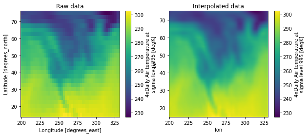
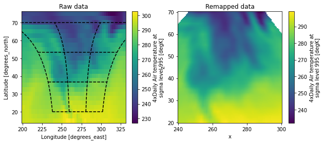
我们的高级插值可用于将数据重新映射到新坐标 考虑二维平面上的新坐标 x 和 z。 重新映射如下面示例所示
# 新坐标
x = np.linspace(240, 300, 100)
z = np.linspace(20, 70, 100)

# 新旧坐标之间的关系
lat = xr.DataArray(
    z,
    dims=['z'],
    coords={'z': z}
)
lon = xr.DataArray(
    (x[:, np.newaxis]-270)/np.cos(z*np.pi/180)+270,
    dims=['x', 'z'],
    coords={'x': x, 'z': z}
)

fig, axes = plt.subplots(ncols=2, figsize=(10, 4))
ds.air.plot(ax=axes[0])

# 在原始坐标中绘制新坐标
for idx in [0, 33, 66, 99]:
     axes[0].plot(
         lon.isel(x=idx),
         lat,
         '--k'
     )
for idx in [0, 33, 66, 99]:
     axes[0].plot(
         *xr.broadcast(
            lon.isel(z=idx),
            lat.isel(z=idx)
         ),
         '--k'
     )

axes[0].set_title('Raw data')

dsi = ds.interp(lon=lon, lat=lat)
dsi.air.plot(ax=axes[1])
axes[1].set_title('Remapped data')

plt.show()