Dask教程:并行和分布式机器学习
本文翻译自 dask-tutorial 项目
Dask-ML 包含用于并行和分布式机器学习的资源。
伸缩类型
Types of scaling
您可能会面临几个明显的伸缩问题。 伸缩策略取决于您面临的问题。
- CPU-Bound:数据适合 RAM,但训练时间太长。许多超参数组合,许多模型的大型集成等。
- 内存限制:数据大于 RAM,并且采样不是一种选择。
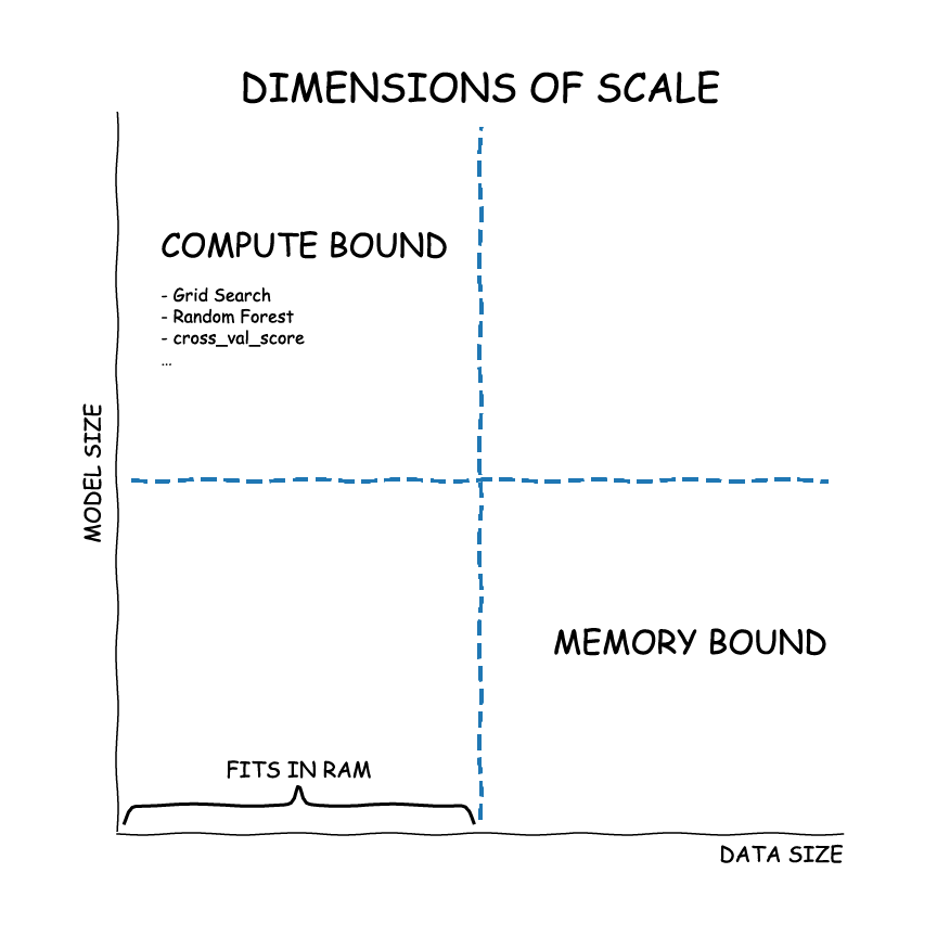
- 对于 in-memory 问题,只需使用 scikit-learn (或您最喜欢的 ML 库)。
- 对于大型模型,请使用
dask_ml.joblib和您最喜欢的 scikit-learn estimator - 对于大型数据集,使用
dask_mlestimator
5 分钟“学会” Scikit-Learn
Scikit-Learn 有很好的、一致的 API。
- 实例化一个
Estimator(例如LinearRegression、RandomForestClassifier等)。 所有模型 超参数 (用户指定的参数,不是估计器学习的参数) 在创建时都会传递给估计器。 - 调用
estimator.fit(X, y)来训练估计器。 - 使用
estimator检查属性、进行预测等。
让我们生成一些随机数据。
from sklearn.datasets import make_classification

X, y = make_classification(
    n_samples=1000,
    n_features=4,
    random_state=0
)
X[:8]
array([[ 1.27815198, -0.41644753,  0.89181112,  0.77129444],
       [ 1.35681817, -1.51465569,  1.82132242,  0.42081175],
       [ 1.53341056,  2.06290707, -1.01967188,  1.87609016],
       [ 0.42064934,  0.05455201,  0.13725671,  0.32493018],
       [-0.88825673, -1.10088618,  0.51393811, -1.05185003],
       [ 0.26413558, -0.42774504,  0.46291997,  0.0326177 ],
       [-1.15189334, -1.43613997,  0.6734141 , -1.36719829],
       [ 0.85289242, -0.74009387,  0.97199307,  0.34318408]])
y[:8]
array([1, 1, 1, 1, 0, 1, 0, 1])
我们训练一个支持向量机分类器
from sklearn.svm import SVC
创建估计器并训练
estimator = SVC(random_state=0)
estimator.fit(X, y)
SVC(random_state=0)
estimator.support_vectors_[:4]
array([[-0.42055907,  1.40271694, -1.32553426,  0.21581905],
       [-0.34484432,  1.48991186, -1.36392417,  0.30301324],
       [-0.63718703,  0.26016267, -0.48744254, -0.36500832],
       [-0.67132345, -0.93017037,  0.46845503, -0.83137829]])
检查准确率
estimator.score(X, y)
0.96
超参数
大多数模型有 超参数 (hyperparameter)。 它们会影响拟合,但会预先指定,而不是在训练期间学习。
estimator = SVC(
    C=0.00001,
    shrinking=False,
    random_state=0
)
estimator.fit(X, y)
estimator.support_vectors_[:4]
array([[-0.88825673, -1.10088618,  0.51393811, -1.05185003],
       [-1.15189334, -1.43613997,  0.6734141 , -1.36719829],
       [-1.5733362 ,  0.21321628, -0.85362176, -1.06050993],
       [-2.549207  , -0.72557246, -0.50971799, -2.11567941]])
estimator.score(X, y)
0.502
超参数优化
有几种方法可以在训练时学习最佳 超参数。
一种是 GridSearchCV。
顾名思义,这会在超参数组合的网格上进行暴力搜索。
from sklearn.model_selection import GridSearchCV
%%time
estimator = SVC(
    gamma="auto",
    random_state=0,
    probability=True
)
param_grid = {
    "C": [0.001, 10.0],
    "kernel": ["rbf", "poly"]
}

grid_search = GridSearchCV(
    estimator,
    param_grid,
    verbose=2,
    cv=2
)
grid_search.fit(X, y)
Fitting 2 folds for each of 4 candidates, totalling 8 fits
[CV] END ................................C=0.001, kernel=rbf; total time=   0.0s
[CV] END ................................C=0.001, kernel=rbf; total time=   0.0s
[CV] END ...............................C=0.001, kernel=poly; total time=   0.0s
[CV] END ...............................C=0.001, kernel=poly; total time=   0.0s
[CV] END .................................C=10.0, kernel=rbf; total time=   0.0s
[CV] END .................................C=10.0, kernel=rbf; total time=   0.0s
[CV] END ................................C=10.0, kernel=poly; total time=   0.0s
[CV] END ................................C=10.0, kernel=poly; total time=   0.0s
Wall time: 448 ms
GridSearchCV(cv=2,
             estimator=SVC(gamma='auto', probability=True, random_state=0),
             param_grid={'C': [0.001, 10.0], 'kernel': ['rbf', 'poly']},
             verbose=2)
使用 scikit-learn 实现单机并行
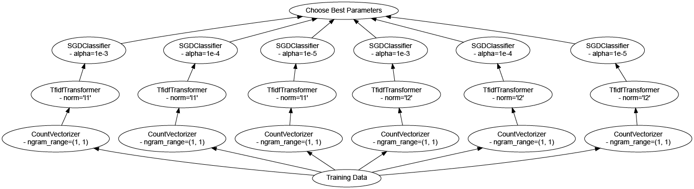
Scikit-Learn 通过 Joblib 具有很好的 单机 (single-machine) 并行性。
任何可以并行操作的 scikit-learn 估计器都会公开一个 n_jobs 关键字,控制将使用的 CPU 内核数。
%%time
grid_search = GridSearchCV(
    estimator,
    param_grid,
    verbose=2,
    cv=2,
    n_jobs=-1
)
grid_search.fit(X, y)
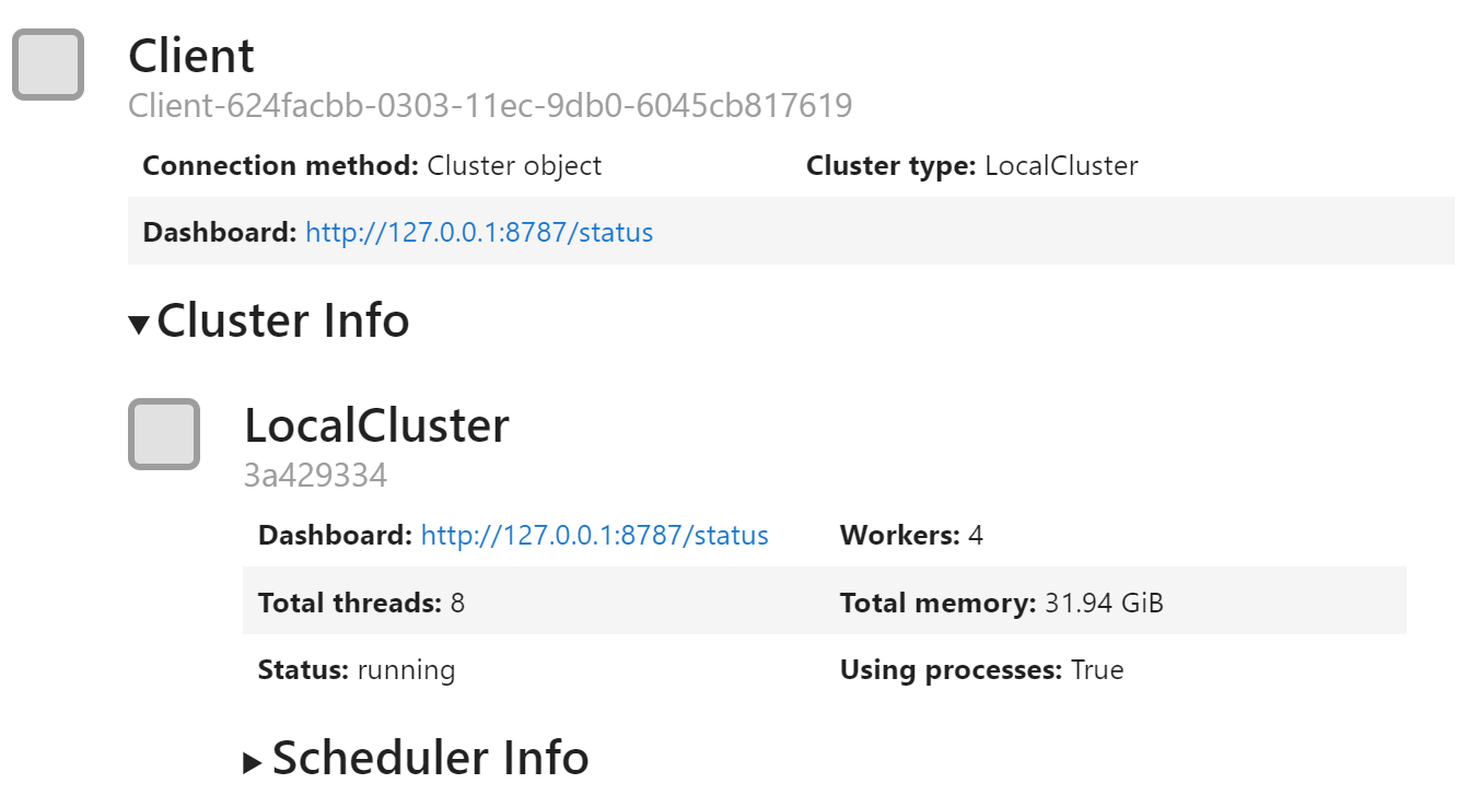
使用 Dask 实现多机并行
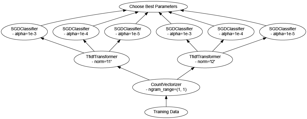
Dask 可以与 scikit-learn (通过 joblib) 通信,以便您的 集群 用于训练模型。
如果您在笔记本电脑上运行,将需要相当长的时间,但 CPU 使用率在此期间将令人满意地接近 100%。
要运行得更快,您需要一个分布式集群。
这意味着在对 Client 的调用中放入一些类似的东西
c = Client("tcp://my.scheduler.address:8786")
可以在此处找到有关创建集群的多种方法的详细信息。
让我们在更大的问题 (更多超参数) 上尝试一下。
import joblib
import dask.distributed

c = dask.distributed.Client()
c
param_grid = {
    "C": [0.001, 0.1, 1.0, 2.5, 10.0],
    # 取消注释此以在集群上进行更大的网格搜索
    # "kernel": ["rbf", "poly", "linear"],
    # "shrinking": [True, False],
}

grid_search = GridSearchCV(
    estimator,
    param_grid,
    verbose=2,
    cv=5,
    n_jobs=-1
)
%%time
with joblib.parallel_backend("dask", scatter=[X, y]):
    grid_search.fit(X, y)
Fitting 5 folds for each of 5 candidates, totalling 25 fits
Wall time: 3.26 s
grid_search.best_params_, grid_search.best_score_
({'C': 2.5}, 0.9629999999999999)
在大型数据集上训练
有时您会想要在比内存更大的数据集上进行训练。
dask-ml 已经实现了估算器,可以很好地处理可能大于机器 RAM 的 dask 数组和数据帧。
import dask.array as da
import dask.delayed
from sklearn.datasets import make_blobs
import numpy as np
我们将使用 scikit-learn 在本地创建一个小型 (随机) 数据集。
n_centers = 12
n_features = 20

X_small, y_small = make_blobs(
    n_samples=1000,
    centers=n_centers,
    n_features=n_features,
    random_state=0
)

centers = np.zeros((n_centers, n_features))

for i in range(n_centers):
    centers[i] = X_small[y_small == i].mean(0)

centers[:4]
array([[ 1.00796679,  4.34582168,  2.15175661,  1.04337835, -1.82115164,
         2.81149666, -1.18757701,  7.74628882,  9.36761449, -2.20570731,
         5.71142324,  0.41084221,  1.34168817,  8.4568751 , -8.59042755,
        -8.35194302, -9.55383028,  6.68605157,  5.34481483,  7.35044606],
       [ 9.49283024,  6.1422784 , -0.97484846,  5.8604399 , -7.61126963,
         2.86555735, -7.25390288,  8.89609285,  0.33510318, -1.79181328,
        -4.66192239,  5.43323887, -0.86162507,  1.3705568 , -9.7904172 ,
         2.3613231 ,  2.20516237,  2.20604823,  8.76464833,  3.47795068],
       [-2.67206588, -1.30103177,  3.98418492, -8.88040428,  3.27735964,
         3.51616445, -5.81395151, -7.42287114, -3.73476887, -2.89520363,
         1.49435043, -1.35811028,  9.91250767, -7.86133474, -5.78975793,
        -6.54897163,  3.08083281, -5.18975209, -0.85563107, -5.06615534],
       [-6.85980599, -7.87144648,  3.33572279, -7.00394241, -5.97224874,
        -2.55638942,  6.36329802, -7.97988653,  6.80059611, -8.14552537,
         9.48255539, -0.67232114,  9.38462699,  2.09067352,  4.80505419,
        -9.14866204, -4.32240399, -7.61670696, -4.14166466, -7.73998277]])
小数据集将成为我们大型随机数据集的模板。
我们将使用 dask.delayed 来应用 sklearn.datasets.make_blobs,以便在我们的工作负载上生成实际的数据集。
n_samples_per_block = 20000
n_blocks = 500

delayeds = [
    dask.delayed(make_blobs)(
        n_samples=n_samples_per_block,
        centers=centers,
        n_features=n_features,
        random_state=i
    )[0] for i in range(n_blocks)
]

arrays = [
    da.from_delayed(
        obj,
        shape=(n_samples_per_block, n_features),
        dtype=X.dtype
    ) for obj in delayeds
]

X = da.concatenate(arrays)
X
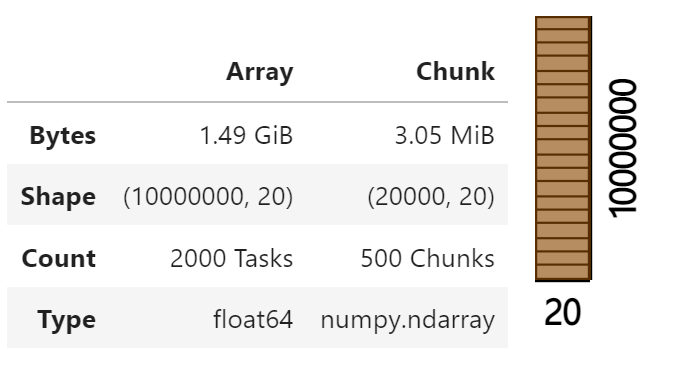
X = X.persist() # 只在集群上运行
Dask-ML 中实现的算法是可扩展的。 它们可以很好地处理大于内存的数据集。
它们遵循 scikit-learn API,因此如果您熟悉 scikit-learn,您会对 Dask-ML 感到宾至如归。
from dask_ml.cluster import KMeans
clf = KMeans(
    init_max_iter=3,
    oversampling_factor=10
)
%time clf.fit(X)
Wall time: 49.1 s
KMeans(init_max_iter=3, oversampling_factor=10)
clf.labels_
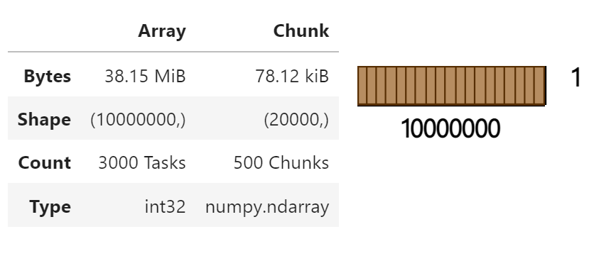
clf.labels_[:10].compute()
array([7, 4, 7, 5, 4, 2, 1, 7, 6, 7])
结束
client.close()
参考
Dask 教程
