GRIB笔记:使用pyinterp实现二维要素场插值
目录
介绍如何使用 pyinterp 实现二维矩阵插值
准备
加载 Python 科学常用库
import numpy as np
import pandas as pd
import xarray as xr
import cartopy.crs as ccrs
import matplotlib.pyplot as plt
使用 nwpc-data 库加载 GRIB2 要素场
from nwpc_data.data_finder import find_local_file
from nwpc_data.grib.eccodes import (
    load_field_from_file,
)
加载 pyinterp 库
import pyinterp
import pyinterp.fill
import pyinterp.backends.xarray
数据
data_path = find_local_file(
    "grapes_gfs_gmf/grib2/orig",
    start_time="2021031100",
    forecast_time="24h"
)
data_path
PosixPath('/g1/COMMONDATA/OPER/NWPC/GRAPES_GFS_GMF/Prod-grib/2021031100/ORIG/gmf.gra.2021031100024.grb2')
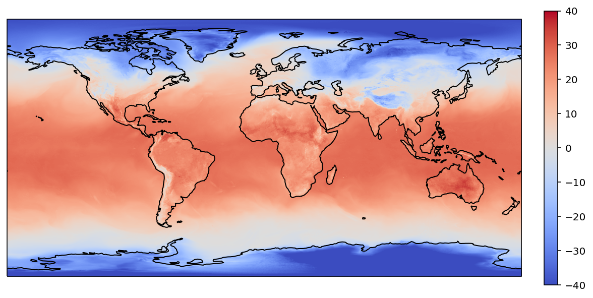
t2m = load_field_from_file(
    data_path,
    parameter="2t",
) - 273.15
t2m
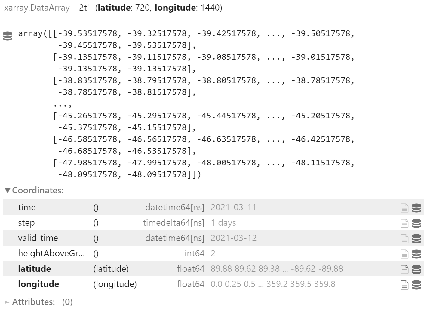
t2m.values.shape
(720, 1440)
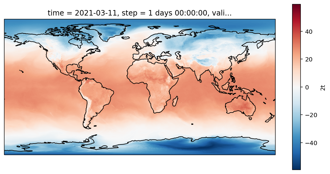
def plot(field):
    fig = plt.figure(figsize=(10, 5))
    ax = plt.axes(projection=ccrs.PlateCarree())
    field.plot(
        ax=ax
    )
    ax.coastlines()
    plt.show()
plot(t2m)
二维网格
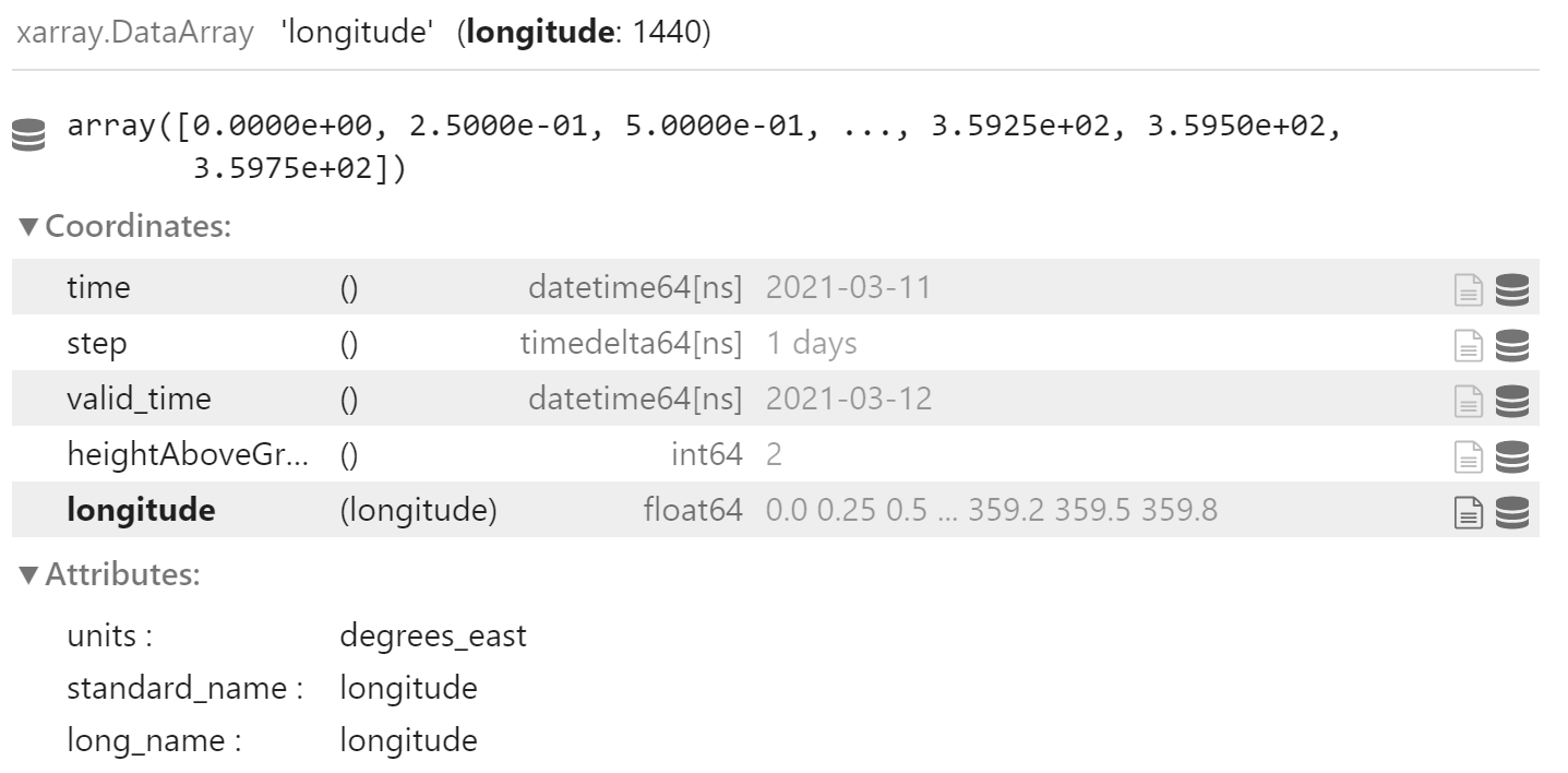
pyinterp.backends.xarray.Grid2D 中默认设置参数 geodetic 为 True,根据维度属性判断经度和纬度:
- 经度:
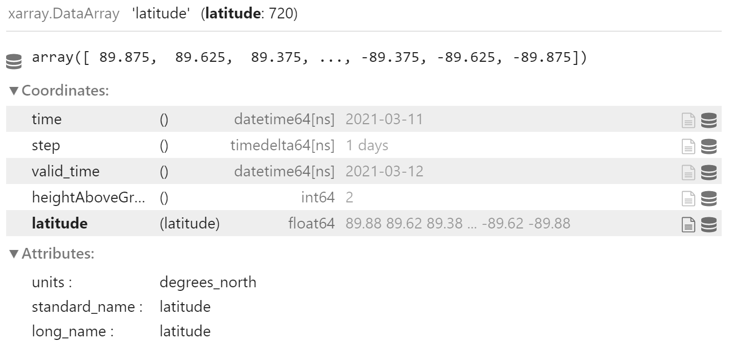
degrees_east,degree_east,degree_E,degrees_E,degreeE - 维度:
degrees_north,degree_north,degree_N,degrees_N,degreeN
t2m.longitude
t2m.latitude
从 xarray.DataArray 中创建二维网格
interpolator = pyinterp.backends.xarray.Grid2D(t2m)
interpolator
<pyinterp.backends.xarray.Grid2D>
Axis:
  x: Axis([0, 0.25, 0.5, ..., 359.5, 359.75], is_circle=true)
  y: Axis([89.875, 89.625, 89.375, ..., -89.625, -89.875], is_circle=false)
Data:
  [[-39.53517578 -39.13517578 -38.83517578 ... -45.26517578 -46.58517578
    -47.98517578]
   [-39.32517578 -39.11517578 -38.79517578 ... -45.29517578 -46.56517578
    -47.99517578]
   [-39.42517578 -39.08517578 -38.80517578 ... -45.44517578 -46.63517578
    -48.00517578]
   ...
   [-39.50517578 -39.01517578 -38.78517578 ... -45.20517578 -46.42517578
    -48.11517578]
   [-39.45517578 -39.13517578 -38.78517578 ... -45.37517578 -46.68517578
    -48.09517578]
   [-39.53517578 -39.13517578 -38.81517578 ... -45.15517578 -46.53517578
    -48.09517578]]
bivariate 实现线性插值
bicubic 实现双三次插值
bivariate
支持多种插值方法 (interpolator),默认使用 bilinear:
bilinearnearestinverse_distance_weighting
单点插值
线性插值
interpolator.bivariate(
    coords={
        "latitude": [39.8062],
        "longitude": [116.4693]
    }
)
array([6.01473833])
最近邻插值
interpolator.bivariate(
    coords={
        "latitude": [39.8062],
        "longitude": [116.4693]
    },
    interpolator="nearest"
)
array([5.86482422])
反距离权重插值
interpolator.bivariate(
    coords={
        "latitude": [39.8062],
        "longitude": [116.4693]
    },
    interpolator="inverse_distance_weighting"
)
array([5.8968783])
多点插值
interpolator.bivariate(
    coords={
        "latitude": [39.8062, 41.80],
        "longitude": [116.4693, 123.40]
    }
)
array([6.01473833, 1.81042422])
网格插值
target_lons = np.arange(0, 360, 0.1)
target_lons
array([0.000e+00, 1.000e-01, 2.000e-01, ..., 3.597e+02, 3.598e+02,
       3.599e+02])
target_lats = np.arange(89.95, -90, -0.1)
target_lats
array([ 89.95, 89.85, 89.75, ..., -89.75, -89.85, -89.95])
target_x, target_y = np.meshgrid(
    target_lons,
    target_lats,
)
target_x.shape, target_y.shape
((1800, 3600), (1800, 3600))
target_values = interpolator.bivariate(
    coords={
        "latitude": target_y.flatten(),
        "longitude": target_x.flatten(),
    }
).reshape(target_x.shape)
target_values
array([[         nan,          nan,          nan, ...,          nan,
                 nan,          nan],
       [-39.49517578, -39.41877578, -39.34237578, ..., -39.48077578,
        -39.49517578, -39.49517578],
       [-39.33517578, -39.28917578, -39.24317578, ..., -39.32717578,
        -39.33517578, -39.33517578],
       ...,
       [-47.28517578, -47.28317578, -47.28117578, ..., -47.33017578,
        -47.31517995, -47.31518829],
       [-47.84517578, -47.84797578, -47.85077578, ..., -47.94217578,
        -47.93918885, -47.93921498],
       [         nan,          nan,          nan, ...,          nan,
                 nan,          nan]])
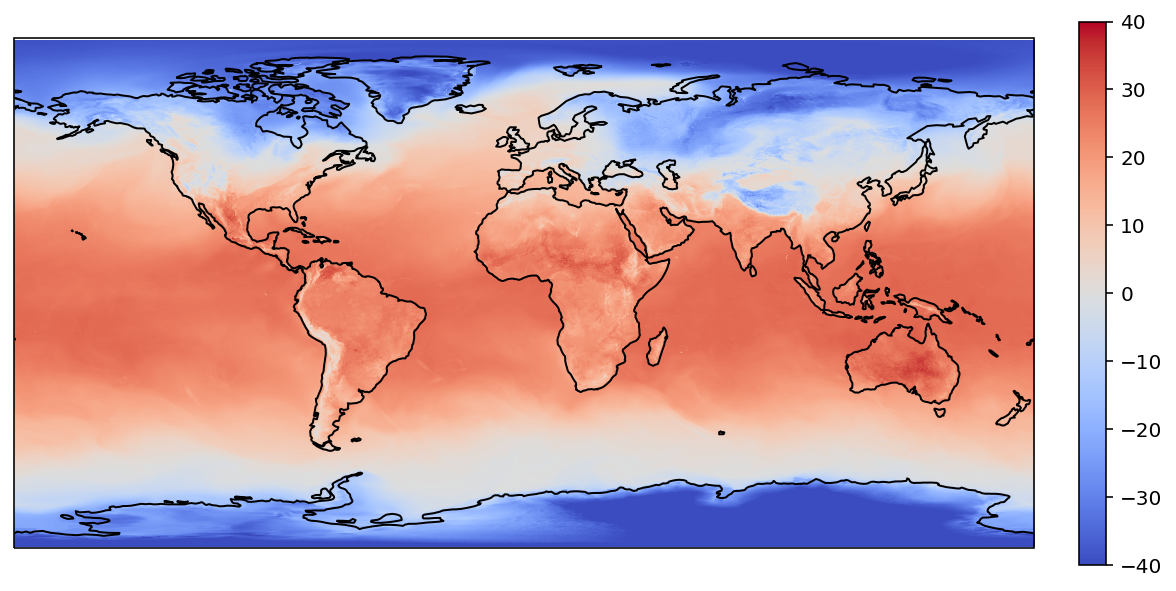
plot_ndarray(
    target_lons,
    target_lats,
    target_values,
)
填充便捷
lons_axis = pyinterp.Axis(target_lons, is_circle=True)
lats_axis = pyinterp.Axis(target_lats, is_circle=False)
lons_axis, lats_axis
(Axis([0, 0.1, 0.2, ..., 359.8, 359.9], is_circle=true),
 Axis([89.95, 89.85, 89.75, ..., -89.85, -89.95], is_circle=false))
target_grid = pyinterp.grid.Grid2D(lats_axis, lons_axis, target_values)
target_values_filled = pyinterp.fill.loess(target_grid)
target_values_filled
array([[-39.26508912, -39.26704999, -39.26875531, ..., -39.3173804 ,
        -39.3239394 , -39.32624573],
       [-39.49517578, -39.41877578, -39.34237578, ..., -39.48077578,
        -39.49517578, -39.49517578],
       [-39.33517578, -39.28917578, -39.24317578, ..., -39.32717578,
        -39.33517578, -39.33517578],
       ...,
       [-47.28517578, -47.28317578, -47.28117578, ..., -47.33017578,
        -47.31517995, -47.31518829],
       [-47.84517578, -47.84797578, -47.85077578, ..., -47.94217578,
        -47.93918885, -47.93921498],
       [-47.2850487 , -47.28724724, -47.29283614, ..., -47.33904643,
        -47.33726795, -47.33307541]])
bicubic
双三次插值
支持多种插值方法 (fitting_model),默认使用 bicubic:
linearbicubicpolynomialc_splinec_spline_periodicakimaakima_periodicsteffen
GSL 库要求作为严格递增,设置 increasing_axes=True 选项翻转降序的维度
interpolator_cubic = pyinterp.backends.xarray.Grid2D(
    t2m,
    increasing_axes=True
)
interpolator_cubic
<pyinterp.backends.xarray.Grid2D>
Axis:
  x: Axis([0, 0.25, 0.5, ..., 359.5, 359.75], is_circle=true)
  y: Axis([-89.875, -89.625, -89.375, ..., 89.625, 89.875], is_circle=false)
Data:
  [[-47.98517578 -46.58517578 -45.26517578 ... -38.83517578 -39.13517578
    -39.53517578]
   [-47.99517578 -46.56517578 -45.29517578 ... -38.79517578 -39.11517578
    -39.32517578]
   [-48.00517578 -46.63517578 -45.44517578 ... -38.80517578 -39.08517578
    -39.42517578]
   ...
   [-48.11517578 -46.42517578 -45.20517578 ... -38.78517578 -39.01517578
    -39.50517578]
   [-48.09517578 -46.68517578 -45.37517578 ... -38.78517578 -39.13517578
    -39.45517578]
   [-48.09517578 -46.53517578 -45.15517578 ... -38.81517578 -39.13517578
    -39.53517578]]
单点插值
interpolator_cubic.bicubic(
    coords={
        "latitude": [39.8062],
        "longitude": [116.4693]
    }
)
array([6.23166967])
多点插值
interpolator_cubic.bicubic(
    coords={
        "latitude": [39.8062, 41.80],
        "longitude": [116.4693, 123.40]
    }
)
array([6.23166967, 1.92946281])
网格插值
target_x_cubic, target_y_cubic = np.meshgrid(
    target_lons,
    target_lats[::-1],
)
target_x_cubic, target_y_cubic
(array([[0.000e+00, 1.000e-01, 2.000e-01, ..., 3.597e+02, 3.598e+02,
         3.599e+02],
        [0.000e+00, 1.000e-01, 2.000e-01, ..., 3.597e+02, 3.598e+02,
         3.599e+02],
        [0.000e+00, 1.000e-01, 2.000e-01, ..., 3.597e+02, 3.598e+02,
         3.599e+02],
        ...,
        [0.000e+00, 1.000e-01, 2.000e-01, ..., 3.597e+02, 3.598e+02,
         3.599e+02],
        [0.000e+00, 1.000e-01, 2.000e-01, ..., 3.597e+02, 3.598e+02,
         3.599e+02],
        [0.000e+00, 1.000e-01, 2.000e-01, ..., 3.597e+02, 3.598e+02,
         3.599e+02]]),
 array([[-89.95, -89.95, -89.95, ..., -89.95, -89.95, -89.95],
        [-89.85, -89.85, -89.85, ..., -89.85, -89.85, -89.85],
        [-89.75, -89.75, -89.75, ..., -89.75, -89.75, -89.75],
        ...,
        [ 89.75,  89.75,  89.75, ...,  89.75,  89.75,  89.75],
        [ 89.85,  89.85,  89.85, ...,  89.85,  89.85,  89.85],
        [ 89.95,  89.95,  89.95, ...,  89.95,  89.95,  89.95]]))
target_values_cubic = interpolator_cubic.bicubic(
    coords={
        "latitude": target_y_cubic.flatten(),
        "longitude": target_x_cubic.flatten(),
    }
).reshape(target_y_cubic.shape)[::-1,]
target_values_cubic
array([[nan, nan, nan, ..., nan, nan, nan],
       [nan, nan, nan, ..., nan, nan, nan],
       [nan, nan, nan, ..., nan, nan, nan],
       ...,
       [nan, nan, nan, ..., nan, nan, nan],
       [nan, nan, nan, ..., nan, nan, nan],
       [nan, nan, nan, ..., nan, nan, nan]])
plot_ndarray(
    target_lons,
    target_lats,
    target_values_cubic,
)
boundary 选项处理边界点,默认使用 nan 填充
注:笔者测试设置 boundary 选项时会出错,尚未找到合适用法来填充边界值
讨论
我使用的 pyinterp 版本是 0.6.1,上文使用 xarray 的函数返回结果是 numpy 数组,而不是 xarray 对象。 我觉得后续最好能提供完整支持 xarray 的 API。
参考
pyinterp 文档:
https://pangeo-pyinterp.readthedocs.io/en/latest/index.html
GRIB 2 数据插值
