GRIB笔记:使用scipy实现二维要素场插值
介绍 scipy.interpolate 包中几种可用于二维矩阵插值的函数
https://docs.scipy.org/doc/scipy/reference/interpolate.html
本文仅简要介绍函数用法,而不比较各种插值类型。
准备
加载 Python 常用科学库
import numpy as np
import pandas as pd
import xarray as xr
import matplotlib.pyplot as plt
import cartopy.crs as ccrs
使用 eccodes 包解码 GRIB2 文件
import eccodes
使用 nwpc-data 库查找数据文件,并加载要素场
from nwpc_data.data_finder import find_local_file
from nwpc_data.grib.eccodes import (
    load_message_from_file
)
数据
使用 GRAPES GFS 全球预报模式系统生成的原始分辨率 GRIB2 产品,分辨率为 0.25 度,网格大小 1440 * 720
data_path = find_local_file(
    "grapes_gfs_gmf/grib2/orig",
    start_time="2021031100",
    forecast_time="24h"
)
data_path
PosixPath('/g1/COMMONDATA/OPER/NWPC/GRAPES_GFS_GMF/Prod-grib/2021031100/ORIG/gmf.gra.2021031100024.grb2')
使用 load_message_from_file() 函数加载 2 米温度场,返回用于 eccodes 包的 GRIB handler 对象
t2m_message = load_message_from_file(
    data_path,
    parameter="2t",
)
t2m_message
93839271854560
网格
GRAPES GFS 模式的 GRIB 2 数据中 scanningMode 值为 0
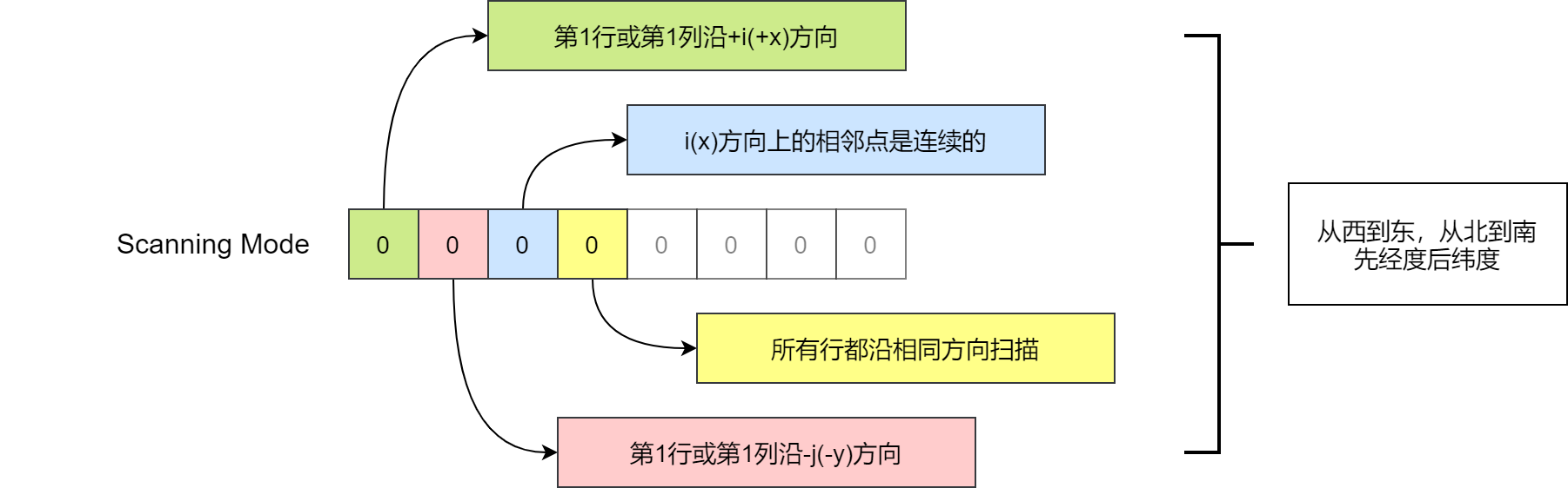
scanningMode 值说明
数据值沿纬度 (即沿行) 保存,从西到东,从北到南排列
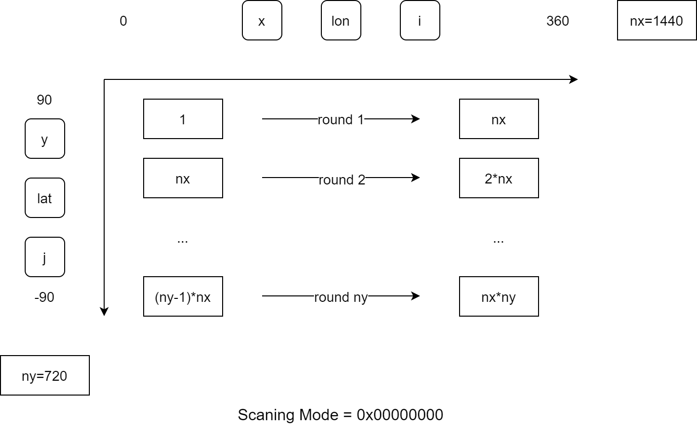
GRAPES 系列模式 GRIB 2 要素场数据值保存示意图
维度信息
读取维度信息,包括:
- 起始点
- 终止点
- 增量
- 数量
经度从 0 到 359.75,间隔 0.25,总计 1440 个值
left_lon = eccodes.codes_get(t2m_message, 'longitudeOfFirstGridPointInDegrees')
right_lon = eccodes.codes_get(t2m_message, 'longitudeOfLastGridPointInDegrees')
lon_step = eccodes.codes_get(t2m_message, 'iDirectionIncrementInDegrees')
nx = eccodes.codes_get(t2m_message, 'Ni')
left_lon, right_lon, lon_step, nx
(0.0, 359.75, 0.25, 1440)
纬度从 89.875 到 -89.875,间隔 0.25,总计 720 个值
top_lat = eccodes.codes_get(t2m_message, 'latitudeOfFirstGridPointInDegrees')
bottom_lat = eccodes.codes_get(t2m_message, 'latitudeOfLastGridPointInDegrees')
lat_step = eccodes.codes_get(t2m_message, 'jDirectionIncrementInDegrees')
ny = eccodes.codes_get(t2m_message, 'Nj')
top_lat, bottom_lat, lat_step, ny
(89.875, -89.875, 0.25, 720)
原始网格
0.25x0.25
为每个维度生成坐标值序列
lons = np.linspace(
    left_lon, right_lon, nx,
    endpoint=True
)
lats = np.linspace(
    top_lat, bottom_lat, ny,
    endpoint=True
)
lons[:10], lats[:10]
(array([0.  , 0.25, 0.5 , 0.75, 1.  , 1.25, 1.5 , 1.75, 2.  , 2.25]),
 array([89.875, 89.625, 89.375, 89.125, 88.875, 88.625, 88.375, 88.125,
        87.875, 87.625]))
orig_x, orig_y = np.meshgrid(lons, lats)
orig_x.shape, orig_y.shape
((720, 1440), (720, 1440))
orig_x, orig_y
(array([[0.0000e+00, 2.5000e-01, 5.0000e-01, ..., 3.5925e+02, 3.5950e+02,
         3.5975e+02],
        [0.0000e+00, 2.5000e-01, 5.0000e-01, ..., 3.5925e+02, 3.5950e+02,
         3.5975e+02],
        [0.0000e+00, 2.5000e-01, 5.0000e-01, ..., 3.5925e+02, 3.5950e+02,
         3.5975e+02],
        ...,
        [0.0000e+00, 2.5000e-01, 5.0000e-01, ..., 3.5925e+02, 3.5950e+02,
         3.5975e+02],
        [0.0000e+00, 2.5000e-01, 5.0000e-01, ..., 3.5925e+02, 3.5950e+02,
         3.5975e+02],
        [0.0000e+00, 2.5000e-01, 5.0000e-01, ..., 3.5925e+02, 3.5950e+02,
         3.5975e+02]]),
 array([[ 89.875,  89.875,  89.875, ...,  89.875,  89.875,  89.875],
        [ 89.625,  89.625,  89.625, ...,  89.625,  89.625,  89.625],
        [ 89.375,  89.375,  89.375, ...,  89.375,  89.375,  89.375],
        ...,
        [-89.375, -89.375, -89.375, ..., -89.375, -89.375, -89.375],
        [-89.625, -89.625, -89.625, ..., -89.625, -89.625, -89.625],
        [-89.875, -89.875, -89.875, ..., -89.875, -89.875, -89.875]]))
目标网格
0.1x0.1
target_lons = np.arange(0, 360, 0.1)
target_lons
array([0.000e+00, 1.000e-01, 2.000e-01, ..., 3.597e+02, 3.598e+02,
       3.599e+02])
target_lats = np.arange(89.95, -90, -0.1)
target_lats
array([ 89.95, 89.85, 89.75, ..., -89.75, -89.85, -89.95])
target_x, target_y = np.meshgrid(
    target_lons,
    target_lats,
)
target_x.shape, target_y.shape
((1800, 3600), (1800, 3600))
target_x, target_y
(array([[0.000e+00, 1.000e-01, 2.000e-01, ..., 3.597e+02, 3.598e+02,
         3.599e+02],
        [0.000e+00, 1.000e-01, 2.000e-01, ..., 3.597e+02, 3.598e+02,
         3.599e+02],
        [0.000e+00, 1.000e-01, 2.000e-01, ..., 3.597e+02, 3.598e+02,
         3.599e+02],
        ...,
        [0.000e+00, 1.000e-01, 2.000e-01, ..., 3.597e+02, 3.598e+02,
         3.599e+02],
        [0.000e+00, 1.000e-01, 2.000e-01, ..., 3.597e+02, 3.598e+02,
         3.599e+02],
        [0.000e+00, 1.000e-01, 2.000e-01, ..., 3.597e+02, 3.598e+02,
         3.599e+02]]),
 array([[ 89.95,  89.95,  89.95, ...,  89.95,  89.95,  89.95],
        [ 89.85,  89.85,  89.85, ...,  89.85,  89.85,  89.85],
        [ 89.75,  89.75,  89.75, ...,  89.75,  89.75,  89.75],
        ...,
        [-89.75, -89.75, -89.75, ..., -89.75, -89.75, -89.75],
        [-89.85, -89.85, -89.85, ..., -89.85, -89.85, -89.85],
        [-89.95, -89.95, -89.95, ..., -89.95, -89.95, -89.95]]))
数据值
将单位转为摄氏度
维度 (720, 1440)
values = eccodes.codes_get_values(t2m_message).reshape(ny, nx) - 273.15
values.shape
(720, 1440)
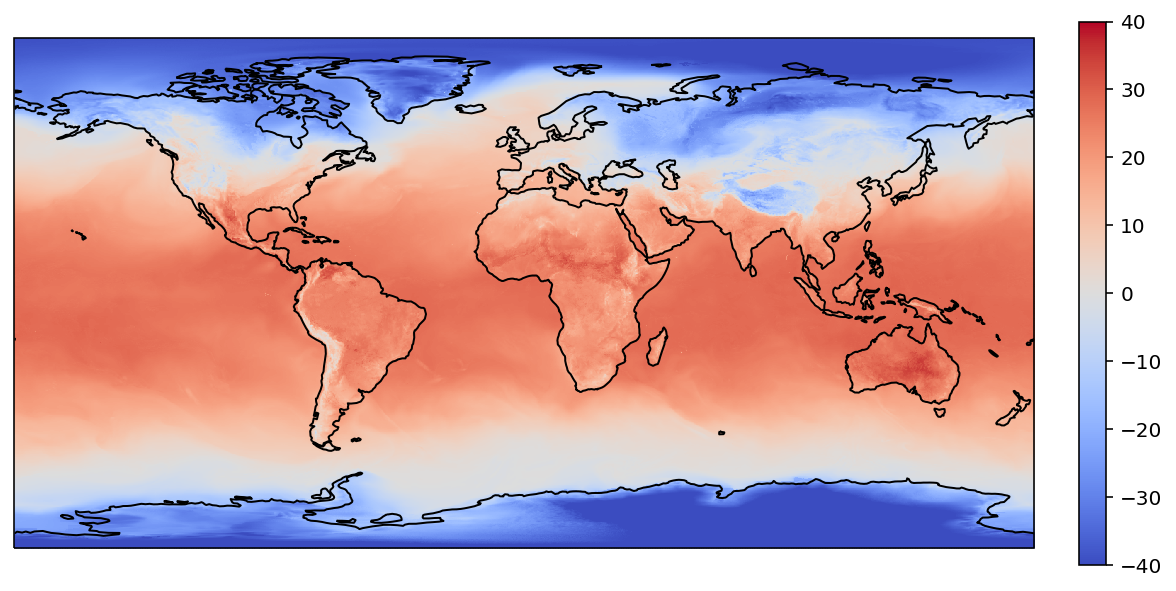
绘图
def plot(lons, lats, values):
    fig = plt.figure(figsize=(10, 5))
    ax = plt.axes(
        projection=ccrs.PlateCarree()
    )
    p = ax.pcolormesh(
        lons, lats, values,
        shading='nearest',
        cmap="coolwarm",
        vmin=-40, vmax=40
    )
    fig.colorbar(p, fraction=0.046, pad=0.04)
    ax.coastlines()
    plt.show()
plot(lons, lats, values)
gribdata
from scipy.interpolate import griddata
griddata() 函数用于插值非结构化 D-D 数据 (unstructure D-D data)
https://docs.scipy.org/doc/scipy/reference/generated/scipy.interpolate.griddata.html
支持多种插值方法 (method),默认使用 linear:
nearest:最近邻插值,NearestNDInterpolatorlinear:线性插值,LinearNDInterpolatorcubic(1-D):三次样条插值cubic(2-D):分段三次,连续可微 (C1),近似曲率最小的多项式曲面,CloughTocher2DInterpolator
单点插值
在本例中:
- 原始网格:([p1_y, p2_y, … , pn_y], [p1_x, p2_x, … , pn_x])
- 原始数据:(p1, p2, …, pn)
- 目标点:经度 116.4693,纬度 39.8062
- 目标数据:一维数组 (1个值)
griddata(
  (orig_y.ravel(), orig_x.ravel()),
  values.ravel(),
  (39.8062, 116.4693),
  method='linear'
)
array(5.96573622)
多点插值
在本例中:
- 原始网格:([p1_y, p2_y, … , pn_y], [p1_x, p2_x, … , pn_x])
- 原始数据:(p1, p2, …, pn)
- 目标点
- 经度 116.4693,纬度 39.8062
- 经度 123.40,纬度 41.80
- 目标数据:一维数组 (2个值)
griddata(
  (orig_y.ravel(), orig_x.ravel()),
  values.ravel(),
  ([39.8062, 41.80], [116.4693, 123.40]),
  method='linear'
)
array([5.96573622, 2.05882422])
网格插值
在本例中:
- 原始网格:([p1_y, p2_y, … , pn_y], [p1_x, p2_x, … , pn_x])
- 原始数据:(p1, p2, …, pn)
- 目标网格:
meshgrid()函数输出的二维坐标值 - 目标数据:二维矩阵
target_values = griddata(
  (orig_y.ravel(), orig_x.ravel()),
  values.ravel(),
  (target_y, target_x),
  method='linear'
)
target_values.shape
(1800, 3600)
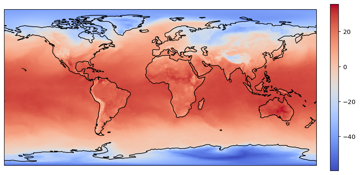
绘图
plot(target_lons, target_lats, target_values)

interp2d
from scipy.interpolate import interp2d
二维网格插值
https://docs.scipy.org/doc/scipy/reference/generated/scipy.interpolate.interp2d.html
支持多种插值方法 (kind),默认为 linear:
linear:线性插值cubic:三次样条插值quintic:五次样条插值
构造插值对象
本例的数据是规则网格数据,所以
- x 设置为列坐标值 (即经度
lons) - y 设置为行坐标值 (即纬度
lats) - z 为二维矩阵
values
注意:本文方法中仅有该函数的 x 对应二维矩阵的列,即 lons。
其余方法中 x 均表示 values 中的第一个维度,即 lats
f_i2d = interp2d(
    lons,
    lats,
    values,
    kind="linear"
)
单点插值
f_i2d(116.4693, 39.8062)
array([6.01473833])
多点插值
interp2d() 返回的对象仅支持对坐标网格的插值
网格插值
注:interp2d.__call__() 方法默认会对坐标值进行排序,所以这里传递翻转后的纬度坐标,并翻转插值结果矩阵的第 1 个维度
i2d_values = f_i2d(
    target_lons,
    target_lats[::-1],
)[::-1, :]
i2d_values.shape
(1800, 3600)
plot(target_lons, target_lats, i2d_values)

interpn
from scipy.interpolate import interpn
规则网格的多维插值
https://docs.scipy.org/doc/scipy/reference/generated/scipy.interpolate.interpn.html
支持多种插值方法 (method),默认为 linear:
linear:线性插值nearest:最近邻插值splinef2d:样条插值,仅支持二维数据
单点插值
在本例中:
- 原始网格:每个维度的坐标值 (按数据维度排序,所以是 lat 和 lon),要求递增
- 原始数据:二维数组
- 目标网格:坐标值
- 目标数据:一维数组
interpn(
    (lats[::-1], lons),
    values[::-1,:],
    [39.8062, 116.4693]
)
array([6.01473833])
多点插值
在本例中:
- 原始数据:二维数组
- 目标网格:坐标数组,每个值表示一组坐标
- 目标数据:一维数组
interpn(
    (lats[::-1], lons),
    values[::-1,:],
    [
        [39.8062, 116.4693],
        [41.80, 123.40],
    ]
)
array([6.01473833, 1.81042422])
网格插值
在本例中:
- 原始网格:每个维度的坐标值,顺序与
values维度一致,要求递增 - 原始数据:二维矩阵
- 目标网格:
meshgrid()函数输出的二维坐标值 - 目标数据:二维矩阵
ipn_values = interpn(
    (lats[::-1], lons),
    values[::-1,:],
    (target_y, target_x),
    bounds_error=False,
    fill_value=None
)
ipn_values
array([[-39.65517578, -39.54837578, -39.44157578, ..., -39.63437578,
        -39.67597578, -39.71757578],
       [-39.49517578, -39.41877578, -39.34237578, ..., -39.48077578,
        -39.50957578, -39.53837578],
       [-39.33517578, -39.28917578, -39.24317578, ..., -39.32717578,
        -39.34317578, -39.35917578],
       ...,
       [-47.28517578, -47.28317578, -47.28117578, ..., -47.33017578,
        -47.30017578, -47.27017578],
       [-47.84517578, -47.84797578, -47.85077578, ..., -47.94217578,
        -47.93617578, -47.93017578],
       [-48.40517578, -48.41277578, -48.42037578, ..., -48.55417578,
        -48.57217578, -48.59017578]])
plot(target_lons, target_lats, ipn_values)

RegularGridInterpolator
from scipy.interpolate import RegularGridInterpolator
在任意维度的规则网格上进行插值
https://docs.scipy.org/doc/scipy/reference/generated/scipy.interpolate.RegularGridInterpolator.html
支持多种插值方法,默认为 linear:
linear:线性插值nearest:最近邻插值
rgi = RegularGridInterpolator(
    (lats[::-1], lons),
    values[::-1,:],
    bounds_error=False,
    fill_value=None
)
单点插值
rgi([39.8062, 116.4693])
array([6.01473833])
__call__() 方法也接收 method 参数,每次计算时指定插值类型
rgi([39.8062, 116.4693], "nearest")
array([5.86482422])
多点插值
rgi([
    [39.8062, 116.4693],
    [41.80, 123.40]
])
array([6.01473833, 1.81042422])
网格插值
注意:list 与 tuple 的区别
rgi_values = rgi(
    (target_y, target_x)
)
rgi_values
array([[-39.65517578, -39.54837578, -39.44157578, ..., -39.63437578,
        -39.67597578, -39.71757578],
       [-39.49517578, -39.41877578, -39.34237578, ..., -39.48077578,
        -39.50957578, -39.53837578],
       [-39.33517578, -39.28917578, -39.24317578, ..., -39.32717578,
        -39.34317578, -39.35917578],
       ...,
       [-47.28517578, -47.28317578, -47.28117578, ..., -47.33017578,
        -47.30017578, -47.27017578],
       [-47.84517578, -47.84797578, -47.85077578, ..., -47.94217578,
        -47.93617578, -47.93017578],
       [-48.40517578, -48.41277578, -48.42037578, ..., -48.55417578,
        -48.57217578, -48.59017578]])
plot(target_lons, target_lats, rgi_values)
RectBivariateSpline
from scipy.interpolate import RectBivariateSpline
矩形网格上的双变量样条曲线逼近。 可以用于平滑和插值。
https://docs.scipy.org/doc/scipy/reference/generated/scipy.interpolate.RectBivariateSpline.html
使用原始数据生成插值对象
rbs = RectBivariateSpline(
    lats[::-1],
    lons,
    values[::-1,:],
    bbox=[-90, 90, 0, 360]
)
单点插值
rbs(39.8062, 116.4693, grid=False)
array(6.23634576)
多点插值
rbs(
    [39.8062, 41.80],
    [116.4693, 123.40],
    grid=False
)
array([6.23634576, 1.92345256])
网格插值
注意:坐标数值必须递增,所以需要翻转纬度
rbs_values = rbs(
    target_lats[::-1],
    target_lons
)[::-1, :]
rbs_values
array([[-39.65647327, -39.4122316 , -39.30781309, ..., -39.48948305,
        -39.80390168, -40.40971356],
       [-39.49414583, -39.39493193, -39.33652311, ..., -39.4829563 ,
        -39.52644163, -39.59177416],
       [-39.33028553, -39.30692735, -39.27675433, ..., -39.37693786,
        -39.29850376, -39.11968022],
       ...,
       [-47.19133329, -47.17869032, -47.20909318, ..., -47.3582264 ,
        -47.09404318, -46.55727764],
       [-47.80334361, -47.81114554, -47.82461448, ..., -47.93604971,
        -47.88091889, -47.77361993],
       [-48.62132701, -48.58439762, -48.54275408, ..., -48.49944652,
        -49.00063039, -50.09441434]])
绘图
plot(target_lons, target_lats, rbs_values)

总结
| 方法 | 插值类型 | 单点插值 | 多点插值 | 网格插值 |
|---|---|---|---|---|
gribdata | nearest, linear, cubic | ✔️ | ✔️ | ✔️ |
interp2d | linear, cubic, quintic | ✔️ | ❌ | ✔️ |
interpn | nearest, linear, splinef2d | ✔️ | ✔️ | ✔️ |
RegularGridInterpolator | nearest, linear | ✔️ | ✔️ | ✔️ |
RectBivariateSpline | ✔️ | ✔️ | ✔️ |
参考
scipy.interpolate 包文档:
https://docs.scipy.org/doc/scipy/reference/interpolate.html
GRIB 2 数据插值
