R语言实战:主成分分析和因子分析
本文内容来自《R 语言实战》(R in Action, 2nd),有部分修改
主成分分析 (PCA):一种数据降维技巧,将大量相关变量转化为一组很少的不相关变量,这些无关变量被称为主成分。
探索性因子分析 (EDA):用来发现一组变量的潜在结构的一系列方法,通过寻找一组更小的、潜在的或隐藏的结构来解释已观测到的、显式的变量间的关系。
R 中的主成分和因子分析
library(psych)
常见步骤:
- 数据预处理。输入原始数据矩阵或者相关系数矩阵给
principal()和fa()函数 - 选择因子模型
- 判断要选择的主成分/因子数目
- 选择主成分/因子
- 旋转主成分/因子
- 解释结果
- 计算主成分或因子得分
主成分分析
head(USJudgeRatings)
               CONT INTG DMNR DILG CFMG DECI PREP FAMI ORAL WRIT PHYS RTEN
AARONSON,L.H.   5.7  7.9  7.7  7.3  7.1  7.4  7.1  7.1  7.1  7.0  8.3  7.8
ALEXANDER,J.M.  6.8  8.9  8.8  8.5  7.8  8.1  8.0  8.0  7.8  7.9  8.5  8.7
ARMENTANO,A.J.  7.2  8.1  7.8  7.8  7.5  7.6  7.5  7.5  7.3  7.4  7.9  7.8
BERDON,R.I.     6.8  8.8  8.5  8.8  8.3  8.5  8.7  8.7  8.4  8.5  8.8  8.7
BRACKEN,J.J.    7.3  6.4  4.3  6.5  6.0  6.2  5.7  5.7  5.1  5.3  5.5  4.8
BURNS,E.B.      6.2  8.8  8.7  8.5  7.9  8.0  8.1  8.0  8.0  8.0  8.6  8.6
判断主成分的个数
Kaiser-Harris 准则
Cattell 碎石检验
平行分析
fa.parallel(
  USJudgeRatings[,-1],
  fa="pc",
  n.iter=100,
  show.legend=TRUE,
  main="Scree plot with parallel analysis"
)
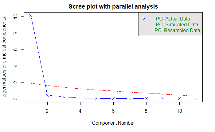
基于观测特征值的碎石检验:线段和 x 符号
根据 100 个随机数据矩阵推到出来的特征值均值:虚线
大于 1 的特征值准则:y = 1 的水平线
以上三种准则都表明选择一个主成分即可保留数据集的大部分信息
提取主成分
USJudgeRatings
提取一个未旋转的主成分
pc <- principal(
  USJudgeRatings[,-1],
  nfractors=1
)
pc
Principal Components Analysis
Call: principal(r = USJudgeRatings[, -1], nfractors = 1)
Standardized loadings (pattern matrix) based upon correlation matrix
      PC1   h2     u2 com
INTG 0.92 0.84 0.1565   1
DMNR 0.91 0.83 0.1663   1
DILG 0.97 0.94 0.0613   1
CFMG 0.96 0.93 0.0720   1
DECI 0.96 0.92 0.0763   1
PREP 0.98 0.97 0.0299   1
FAMI 0.98 0.95 0.0469   1
ORAL 1.00 0.99 0.0091   1
WRIT 0.99 0.98 0.0196   1
PHYS 0.89 0.80 0.2013   1
RTEN 0.99 0.97 0.0275   1

                 PC1
SS loadings    10.13
Proportion Var  0.92

Mean item complexity =  1
Test of the hypothesis that 1 component is sufficient.

The root mean square of the residuals (RMSR) is  0.04
 with the empirical chi square  6.21  with prob <  1

Fit based upon off diagonal values = 1
PC1:成分载荷,观测变量与主成分的相关系数。PC1 表示第一个主成分
h2:公因子方差,主成分对每个变量的方差解释度
u2:成分唯一性,方差无法被主成分解释的比例,1 - h2
SS loadings:与主成分相关的特征值
Proportion Var:每个主成分对整个数据集的解释程度
Harman23.cor
数据集由变量的相关系数组成
head(Harman23.cor)
$cov
               height arm.span forearm lower.leg weight bitro.diameter
height          1.000    0.846   0.805     0.859  0.473          0.398
arm.span        0.846    1.000   0.881     0.826  0.376          0.326
forearm         0.805    0.881   1.000     0.801  0.380          0.319
lower.leg       0.859    0.826   0.801     1.000  0.436          0.329
weight          0.473    0.376   0.380     0.436  1.000          0.762
bitro.diameter  0.398    0.326   0.319     0.329  0.762          1.000
chest.girth     0.301    0.277   0.237     0.327  0.730          0.583
chest.width     0.382    0.415   0.345     0.365  0.629          0.577
               chest.girth chest.width
height               0.301       0.382
arm.span             0.277       0.415
forearm              0.237       0.345
lower.leg            0.327       0.365
weight               0.730       0.629
bitro.diameter       0.583       0.577
chest.girth          1.000       0.539
chest.width          0.539       1.000

$center
[1] 0 0 0 0 0 0 0 0

$n.obs
[1] 305
fa.parallel(
  Harman23.cor$cov,
  n.obs=302,
  fa="pc",
  n.iter=100,
  show.legend=TRUE,
  main="Scree plot with parallel analysis"
)
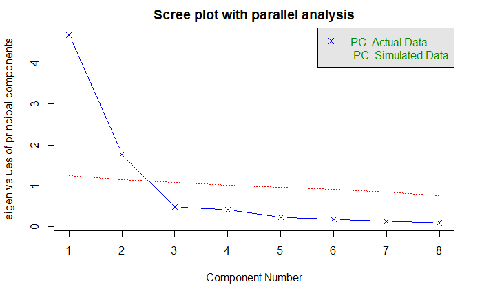
三个准则都建议选择两个主成分
pc <- principal(
  Harman23.cor$cov,
  nfactors=2,
  rotate="none"
)
pc
Principal Components Analysis
Call: principal(r = Harman23.cor$cov, nfactors = 2, rotate = "none")
Standardized loadings (pattern matrix) based upon correlation matrix
                PC1   PC2   h2    u2 com
height         0.86 -0.37 0.88 0.123 1.4
arm.span       0.84 -0.44 0.90 0.097 1.5
forearm        0.81 -0.46 0.87 0.128 1.6
lower.leg      0.84 -0.40 0.86 0.139 1.4
weight         0.76  0.52 0.85 0.150 1.8
bitro.diameter 0.67  0.53 0.74 0.261 1.9
chest.girth    0.62  0.58 0.72 0.283 2.0
chest.width    0.67  0.42 0.62 0.375 1.7

                       PC1  PC2
SS loadings           4.67 1.77
Proportion Var        0.58 0.22
Cumulative Var        0.58 0.81
Proportion Explained  0.73 0.27
Cumulative Proportion 0.73 1.00

Mean item complexity =  1.7
Test of the hypothesis that 2 components are sufficient.

The root mean square of the residuals (RMSR) is  0.05

Fit based upon off diagonal values = 0.99
第一主成分解释 58% 方差,第二主成分解释 22% 方差,两者一共解释 81% 方差
主成分旋转
旋转是将成分载荷阵变得更容易解释的一系列数学方法,尽可能对成分去噪。 方法有两种:
- 正交旋转:使选择的成分保持不相关
- 斜交旋转:让它们变得相关
最流行的是方差极大旋转,是每个成分只由一组有限的变量来解释
rc <- principal(
  Harman23.cor$cov,
  nfactors=2,
  rotate="varimax"
)
rc
Principal Components Analysis
Call: principal(r = Harman23.cor$cov, nfactors = 2, rotate = "varimax")
Standardized loadings (pattern matrix) based upon correlation matrix
                RC1  RC2   h2    u2 com
height         0.90 0.25 0.88 0.123 1.2
arm.span       0.93 0.19 0.90 0.097 1.1
forearm        0.92 0.16 0.87 0.128 1.1
lower.leg      0.90 0.22 0.86 0.139 1.1
weight         0.26 0.88 0.85 0.150 1.2
bitro.diameter 0.19 0.84 0.74 0.261 1.1
chest.girth    0.11 0.84 0.72 0.283 1.0
chest.width    0.26 0.75 0.62 0.375 1.2

                       RC1  RC2
SS loadings           3.52 2.92
Proportion Var        0.44 0.37
Cumulative Var        0.44 0.81
Proportion Explained  0.55 0.45
Cumulative Proportion 0.55 1.00

Mean item complexity =  1.1
Test of the hypothesis that 2 components are sufficient.

The root mean square of the residuals (RMSR) is  0.05

Fit based upon off diagonal values = 0.99
第一个主成分主要由前四个变量解释 (长度变量),第二个主成分主要由后四个变量解释 (容量变量)
获得主成分得分
USJudgeRatings
获得每个观测在某个主成分上的得分
pc <- principal(
  USJudgeRatings[,-1],
  nfactors=1,
  score=TRUE
)
head(pc$scores)
                      PC1
AARONSON,L.H.  -0.1857981
ALEXANDER,J.M.  0.7469865
ARMENTANO,A.J.  0.0704772
BERDON,R.I.     1.1358765
BRACKEN,J.J.   -2.1586211
BURNS,E.B.      0.7669406
律师与法官的接触频数与法官评分间的相关系数 (毫无关联)
cov(USJudgeRatings$CONT, pc$scores)
              PC1
[1,] -0.008294671
Harman23.cor
使用相关系数矩阵时,仅能计算得分系数
rc <- principal(
  Harman23.cor$cov,
  nfactors=2,
  rotate="varimax"
)
round(rc$weights, 2)
                 RC1   RC2
height          0.28 -0.05
arm.span        0.30 -0.08
forearm         0.30 -0.09
lower.leg       0.28 -0.06
weight         -0.06  0.33
bitro.diameter -0.08  0.32
chest.girth    -0.10  0.34
chest.width    -0.04  0.27
探索性因子分析
EFA 目标是通过发掘隐藏在数据下的一组较少的、更为基本的无法观测的变量,来解释一组可供观测变量的相关性。 这些虚拟的、无法观测的变量称作因子。
$$ X_i = a_1F_1 + a_2F_2 + … + a_pF_p + U_i $$
其中 X_i 是第 i 个可观测变量,F_j 是公共因子,p < k,U_i 是 X_i 变量独有的部分,无法被公共因子解释
ability.cov 数据集提供协方差矩阵
ability.cov
$cov
        general picture  blocks   maze reading   vocab
general  24.641   5.991  33.520  6.023  20.755  29.701
picture   5.991   6.700  18.137  1.782   4.936   7.204
blocks   33.520  18.137 149.831 19.424  31.430  50.753
maze      6.023   1.782  19.424 12.711   4.757   9.075
reading  20.755   4.936  31.430  4.757  52.604  66.762
vocab    29.701   7.204  50.753  9.075  66.762 135.292

$center
[1] 0 0 0 0 0 0

$n.obs
[1] 112
使用 cov2cor() 函数将协方差矩阵转为相关系数矩阵
covariances <- ability.cov$cov
correlations <- cov2cor(covariances)
correlations
          general   picture    blocks      maze   reading     vocab
general 1.0000000 0.4662649 0.5516632 0.3403250 0.5764799 0.5144058
picture 0.4662649 1.0000000 0.5724364 0.1930992 0.2629229 0.2392766
blocks  0.5516632 0.5724364 1.0000000 0.4450901 0.3540252 0.3564715
maze    0.3403250 0.1930992 0.4450901 1.0000000 0.1839645 0.2188370
reading 0.5764799 0.2629229 0.3540252 0.1839645 1.0000000 0.7913779
vocab   0.5144058 0.2392766 0.3564715 0.2188370 0.7913779 1.0000000
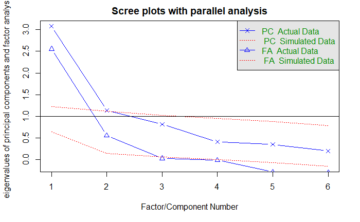
判断需提取的公因子数
fa.parallel(
  correlations,
  n.obs=221,
  fa="both",
  n.iter=100,
  main="Scree plots with parallel analysis"
)
提取公因子
提取两个因子,使用主轴迭代法 (fm="pa") 提取未旋转因子
fa.pa <- fa(
  correlations,
  nfactors=2,
  rotate="none",
  fm="pa"
)
fa.pa
Factor Analysis using method =  pa
Call: fa(r = correlations, nfactors = 2, rotate = "none", fm = "pa")
Standardized loadings (pattern matrix) based upon correlation matrix
         PA1   PA2   h2    u2 com
general 0.75  0.07 0.57 0.432 1.0
picture 0.52  0.32 0.38 0.623 1.7
blocks  0.75  0.52 0.83 0.166 1.8
maze    0.39  0.22 0.20 0.798 1.6
reading 0.81 -0.51 0.91 0.089 1.7
vocab   0.73 -0.39 0.69 0.313 1.5

                       PA1  PA2
SS loadings           2.75 0.83
Proportion Var        0.46 0.14
Cumulative Var        0.46 0.60
Proportion Explained  0.77 0.23
Cumulative Proportion 0.77 1.00

Mean item complexity =  1.5
Test of the hypothesis that 2 factors are sufficient.

The degrees of freedom for the null model are  15  and the objective function was  2.48
The degrees of freedom for the model are 4  and the objective function was  0.07

The root mean square of the residuals (RMSR) is  0.03
The df corrected root mean square of the residuals is  0.06

Fit based upon off diagonal values = 0.99
Measures of factor score adequacy
                                                   PA1  PA2
Correlation of (regression) scores with factors   0.96 0.92
Multiple R square of scores with factors          0.93 0.84
Minimum correlation of possible factor scores     0.86 0.68
两个因子解释 60% 方差
因子旋转
正交旋转
fa.varimax <- fa(
  correlations,
  nfactors=2,
  rotate="varimax",
  fm="pa"
)
fa.varimax
Factor Analysis using method =  pa
Call: fa(r = correlations, nfactors = 2, rotate = "varimax",
    fm = "pa")
Standardized loadings (pattern matrix) based upon correlation matrix
         PA1  PA2   h2    u2 com
general 0.49 0.57 0.57 0.432 2.0
picture 0.16 0.59 0.38 0.623 1.1
blocks  0.18 0.89 0.83 0.166 1.1
maze    0.13 0.43 0.20 0.798 1.2
reading 0.93 0.20 0.91 0.089 1.1
vocab   0.80 0.23 0.69 0.313 1.2

                       PA1  PA2
SS loadings           1.83 1.75
Proportion Var        0.30 0.29
Cumulative Var        0.30 0.60
Proportion Explained  0.51 0.49
Cumulative Proportion 0.51 1.00

Mean item complexity =  1.3
Test of the hypothesis that 2 factors are sufficient.

The degrees of freedom for the null model are  15  and the objective function was  2.48
The degrees of freedom for the model are 4  and the objective function was  0.07

The root mean square of the residuals (RMSR) is  0.03
The df corrected root mean square of the residuals is  0.06

Fit based upon off diagonal values = 0.99
Measures of factor score adequacy
                                                   PA1  PA2
Correlation of (regression) scores with factors   0.96 0.92
Multiple R square of scores with factors          0.91 0.85
Minimum correlation of possible factor scores     0.82 0.71
斜交转轴法,比如 promax
fa.promax <- fa(
  correlations,
  nfactors=2,
  rotate="promax",
  fm="pa"
)
fa.promax
Factor Analysis using method =  pa
Call: fa(r = correlations, nfactors = 2, rotate = "promax", fm = "pa")
Standardized loadings (pattern matrix) based upon correlation matrix
          PA1   PA2   h2    u2 com
general  0.37  0.48 0.57 0.432 1.9
picture -0.03  0.63 0.38 0.623 1.0
blocks  -0.10  0.97 0.83 0.166 1.0
maze     0.00  0.45 0.20 0.798 1.0
reading  1.00 -0.09 0.91 0.089 1.0
vocab    0.84 -0.01 0.69 0.313 1.0

                       PA1  PA2
SS loadings           1.83 1.75
Proportion Var        0.30 0.29
Cumulative Var        0.30 0.60
Proportion Explained  0.51 0.49
Cumulative Proportion 0.51 1.00

 With factor correlations of
     PA1  PA2
PA1 1.00 0.55
PA2 0.55 1.00

Mean item complexity =  1.2
Test of the hypothesis that 2 factors are sufficient.

The degrees of freedom for the null model are  15  and the objective function was  2.48
The degrees of freedom for the model are 4  and the objective function was  0.07

The root mean square of the residuals (RMSR) is  0.03
The df corrected root mean square of the residuals is  0.06

Fit based upon off diagonal values = 0.99
Measures of factor score adequacy
                                                   PA1  PA2
Correlation of (regression) scores with factors   0.97 0.94
Multiple R square of scores with factors          0.93 0.88
Minimum correlation of possible factor scores     0.86 0.77
因子结构矩阵:变量与因子的相关系数
因子模式矩阵:标准化的回归系数矩阵,Standardized loadings
因子关联矩阵:因子相关系数矩阵,factor correlations
正交旋转仅考虑第一项,斜交旋转会考虑全部三项
计算因子结构矩阵 (又称因子载荷阵):F = P * Phi
- F:因子载荷阵
- P:因子模式矩阵
- Phi:因子关联矩阵
fsm <- function(oblique) {
  if (class(oblique)[2] == "fa" & is.null(oblique$Phi)) {
    warning("Object doesn't look like oblique EFA")
  } else {
    P <- unclass(oblique$loading)
    F <- P %*% oblique$Phi
    colnames(F) <- c("PA1", "PA2")
    return (F)
  }
}
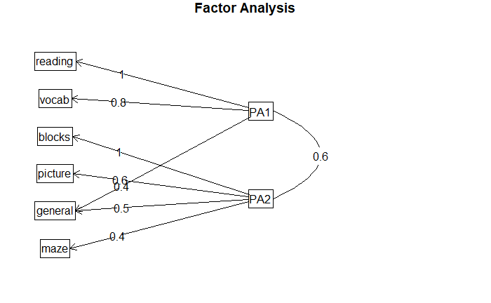
fsm(fa.promax)
              PA1       PA2
general 0.6362443 0.6879280
picture 0.3203301 0.6137902
blocks  0.4293252 0.9089946
maze    0.2491789 0.4496446
reading 0.9510795 0.4587468
vocab   0.8287066 0.4476297
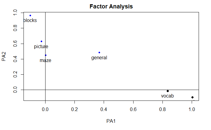
绘图
factor.plot(
  fa.promax,
  labels=rownames(fa.promax$loadings)
)
fa.diagram(
  fa.promax,
  simple=FALSE
)
Harman74.cor 数据集
fa.24tests <- fa(
  Harman74.cor$cov,
  nfactors=4,
  rotate="promax"
)
fa.24tests
Factor Analysis using method =  minres
Call: fa(r = Harman74.cor$cov, nfactors = 4, rotate = "promax")
Standardized loadings (pattern matrix) based upon correlation matrix
                         MR1   MR3   MR2   MR4   h2   u2 com
VisualPerception       -0.08  0.78  0.06 -0.05 0.55 0.45 1.0
Cubes                  -0.02  0.53 -0.02 -0.05 0.23 0.77 1.0
PaperFormBoard          0.00  0.66 -0.16 -0.01 0.34 0.66 1.1
Flags                   0.10  0.60 -0.03 -0.10 0.35 0.65 1.1
GeneralInformation      0.79 -0.02  0.10 -0.05 0.64 0.36 1.0
PargraphComprehension   0.82  0.00 -0.11  0.09 0.68 0.32 1.1
SentenceCompletion      0.91 -0.02  0.03 -0.14 0.73 0.27 1.0
WordClassification      0.54  0.22  0.11 -0.06 0.51 0.49 1.4
WordMeaning             0.89 -0.02 -0.13  0.08 0.74 0.26 1.1
Addition                0.09 -0.39  0.97 -0.01 0.74 0.26 1.3
Code                    0.03 -0.11  0.53  0.29 0.47 0.53 1.7
CountingDots           -0.15  0.09  0.81 -0.11 0.55 0.45 1.1
StraightCurvedCapitals  0.00  0.38  0.55 -0.17 0.51 0.49 2.0
WordRecognition         0.11 -0.15 -0.07  0.65 0.36 0.64 1.2
NumberRecognition      -0.01 -0.03 -0.07  0.61 0.31 0.69 1.0
FigureRecognition      -0.15  0.39 -0.14  0.54 0.45 0.55 2.2
ObjectNumber            0.00 -0.15  0.11  0.66 0.41 0.59 1.2
NumberFigure           -0.21  0.21  0.25  0.42 0.41 0.59 2.8
FigureWord              0.01  0.16  0.07  0.32 0.23 0.77 1.6
Deduction               0.27  0.35 -0.07  0.18 0.42 0.58 2.5
NumericalPuzzles        0.00  0.34  0.38  0.03 0.42 0.58 2.0
ProblemReasoning        0.26  0.33 -0.03  0.17 0.40 0.60 2.5
SeriesCompletion        0.23  0.48  0.09  0.04 0.51 0.49 1.5
ArithmeticProblems      0.27 -0.03  0.45  0.14 0.49 0.51 1.9

                       MR1  MR3  MR2  MR4
SS loadings           3.70 2.95 2.72 2.11
Proportion Var        0.15 0.12 0.11 0.09
Cumulative Var        0.15 0.28 0.39 0.48
Proportion Explained  0.32 0.26 0.24 0.18
Cumulative Proportion 0.32 0.58 0.82 1.00

 With factor correlations of
     MR1  MR3  MR2  MR4
MR1 1.00 0.59 0.47 0.53
MR3 0.59 1.00 0.53 0.59
MR2 0.47 0.53 1.00 0.56
MR4 0.53 0.59 0.56 1.00

Mean item complexity =  1.5
Test of the hypothesis that 4 factors are sufficient.

The degrees of freedom for the null model are  276  and the objective function was  11.44
The degrees of freedom for the model are 186  and the objective function was  1.72

The root mean square of the residuals (RMSR) is  0.04
The df corrected root mean square of the residuals is  0.05

Fit based upon off diagonal values = 0.98
Measures of factor score adequacy
                                                   MR1  MR3  MR2  MR4
Correlation of (regression) scores with factors   0.96 0.93 0.94 0.90
Multiple R square of scores with factors          0.92 0.86 0.89 0.81
Minimum correlation of possible factor scores     0.85 0.72 0.77 0.61
因子得分
fa.promax$weights
               PA1        PA2
general 0.07836571 0.21091463
picture 0.02000694 0.09038071
blocks  0.03662858 0.70209400
maze    0.02700266 0.03453381
reading 0.74276722 0.03012597
vocab   0.17683183 0.03583324
其他与 EFA 相关的包
- FactoMineR
- FAiR
- GPArotation
- nFactors
其他潜变量模型
结构方程模型 (SEM),验证性因子分析 (CFA)
潜类别模型
简单和多重对应分析
多维标度法 (MDS)
参考
https://github.com/perillaroc/r-in-action-study
R 语言实战
