R语言实战:广义线性模型
本文内容来自《R 语言实战》(R in Action, 2nd),有部分修改
广义线性模型和 glm() 函数
标准线性模型:假设 Y 呈正态分布
广义线性模型:假设 Y 服从指数分布族中的一种分布
glm() 函数
基本形式
glm(
  formula,
  family=family(link=function),
  data=data
)
Logistic 回归:用于二值响应变量 (0 和 1)
$$ log_{e}(\frac{\pi}{1-\pi}) = \beta_0 + \sum_{j=1}^{p}\beta_{j}X_{j} $$
glm(
  Y ~ X1 + X2 + X3,
  family=binomial(link="logit"),
  data=mydata
)
泊松回归:适用于在给定时间内响应变量为事件发生数目的情形
$$ log_{e}(\lambda) = \beta_0 + \sum_{j=1}^{p}\beta_{j}X_{j} $$
glm(
  Y ~ X1 + X2 + X3,
  family=possion(link="log"),
  data=mydata
)
标准线性回归:广义线性回归的一种特例
$$ \mu_{Y} = \beta_0 + \sum_{j=1}^{p}\beta_{j}X_{j} $$
glm(
  Y ~ X1 + X2 + X3,
  family=guassian(link="identity"),
  data=mydata
)
与下面代码相同
lm(
  Y ~ X1 + X2 + X3,
  data=mydata
)
连用的函数
summary()coefficients()confint()residuals()anova()plot()predict()deviance()df.residual()
模型拟合和回归诊断
预测值与残差
plot(
  predict(model, type="response"),
  residuals(model, type="deviance")
)
帽子值
plot(hatvalues(model))
学生化残差
plot(rstudent(model))
Cook 距离统计量
plot(cooks.distance(model))
car 包的影像图
library(car)
influencePlot(model)
Logistic 回归
data(Affairs, package="AER")
head(Affairs)
   affairs gender age yearsmarried children religiousness education
4        0   male  37        10.00       no             3        18
5        0 female  27         4.00       no             4        14
11       0 female  32        15.00      yes             1        12
16       0   male  57        15.00      yes             5        18
23       0   male  22         0.75       no             2        17
29       0 female  32         1.50       no             2        17
   occupation rating ynaffair
4           7      4       No
5           6      4       No
11          1      4       No
16          6      5       No
23          6      3       No
29          5      5       No
summary(Affairs)
    affairs          gender         age         yearsmarried    children
 Min.   : 0.000   female:315   Min.   :17.50   Min.   : 0.125   no :171
 1st Qu.: 0.000   male  :286   1st Qu.:27.00   1st Qu.: 4.000   yes:430
 Median : 0.000                Median :32.00   Median : 7.000
 Mean   : 1.456                Mean   :32.49   Mean   : 8.178
 3rd Qu.: 0.000                3rd Qu.:37.00   3rd Qu.:15.000
 Max.   :12.000                Max.   :57.00   Max.   :15.000
 religiousness     education       occupation        rating
 Min.   :1.000   Min.   : 9.00   Min.   :1.000   Min.   :1.000
 1st Qu.:2.000   1st Qu.:14.00   1st Qu.:3.000   1st Qu.:3.000
 Median :3.000   Median :16.00   Median :5.000   Median :4.000
 Mean   :3.116   Mean   :16.17   Mean   :4.195   Mean   :3.932
 3rd Qu.:4.000   3rd Qu.:18.00   3rd Qu.:6.000   3rd Qu.:5.000
 Max.   :5.000   Max.   :20.00   Max.   :7.000   Max.   :5.000
 ynaffair
 No :451
 Yes:150
table(Affairs$affairs)
  0   1   2   3   7  12
451  34  17  19  42  38
生成二值型变量
Affairs$ynaffair <- ifelse(
  Affairs$affairs == 0, 0, 1
)
Affairs$ynaffair <- factor(
  Affairs$ynaffair,
  levels=c(0, 1),
  labels=c("No", "Yes")
)
table(Affairs$ynaffair)
 No Yes
451 150
使用 Logistic 回归拟合
fit_full <- glm(
  ynaffair ~ gender + age + yearsmarried + children +
    religiousness + education + occupation + rating,
  data=Affairs,
  family=binomial()
)
summary(fit_full)
Call:
glm(formula = ynaffair ~ gender + age + yearsmarried + children +
    religiousness + education + occupation + rating, family = binomial(),
    data = Affairs)

Deviance Residuals:
    Min       1Q   Median       3Q      Max
-1.5713  -0.7499  -0.5690  -0.2539   2.5191

Coefficients:
              Estimate Std. Error z value Pr(>|z|)
(Intercept)    1.37726    0.88776   1.551 0.120807
gendermale     0.28029    0.23909   1.172 0.241083
age           -0.04426    0.01825  -2.425 0.015301 *
yearsmarried   0.09477    0.03221   2.942 0.003262 **
childrenyes    0.39767    0.29151   1.364 0.172508
religiousness -0.32472    0.08975  -3.618 0.000297 ***
education      0.02105    0.05051   0.417 0.676851
occupation     0.03092    0.07178   0.431 0.666630
rating        -0.46845    0.09091  -5.153 2.56e-07 ***
---
Signif. codes:  0 ‘***’ 0.001 ‘**’ 0.01 ‘*’ 0.05 ‘.’ 0.1 ‘ ’ 1

(Dispersion parameter for binomial family taken to be 1)

    Null deviance: 675.38  on 600  degrees of freedom
Residual deviance: 609.51  on 592  degrees of freedom
AIC: 627.51

Number of Fisher Scoring iterations: 4
去掉不显著的变量,重新拟合
fit_reduced <- glm(
  ynaffair ~ age + yearsmarried + religiousness + rating,
  data=Affairs,
  family=binomial()
)
summary(fit_reduced)
Call:
glm(formula = ynaffair ~ age + yearsmarried + religiousness +
    rating, family = binomial(), data = Affairs)

Deviance Residuals:
    Min       1Q   Median       3Q      Max
-1.6278  -0.7550  -0.5701  -0.2624   2.3998

Coefficients:
              Estimate Std. Error z value Pr(>|z|)
(Intercept)    1.93083    0.61032   3.164 0.001558 **
age           -0.03527    0.01736  -2.032 0.042127 *
yearsmarried   0.10062    0.02921   3.445 0.000571 ***
religiousness -0.32902    0.08945  -3.678 0.000235 ***
rating        -0.46136    0.08884  -5.193 2.06e-07 ***
---
Signif. codes:  0 ‘***’ 0.001 ‘**’ 0.01 ‘*’ 0.05 ‘.’ 0.1 ‘ ’ 1

(Dispersion parameter for binomial family taken to be 1)

    Null deviance: 675.38  on 600  degrees of freedom
Residual deviance: 615.36  on 596  degrees of freedom
AIC: 625.36

Number of Fisher Scoring iterations: 4
使用卡方检验比较两个模型的效果是否相同
anova(
  fit_reduced,
  fit_full,
  test="Chisq"
)
Analysis of Deviance Table

Model 1: ynaffair ~ age + yearsmarried + religiousness + rating
Model 2: ynaffair ~ gender + age + yearsmarried + children + religiousness +
    education + occupation + rating
  Resid. Df Resid. Dev Df Deviance Pr(>Chi)
1       596     615.36
2       592     609.51  4   5.8474   0.2108
卡方值不显著,说明两个模型预测效果相同,可以用变量较少的模型代替变量较多的模型
诊断图
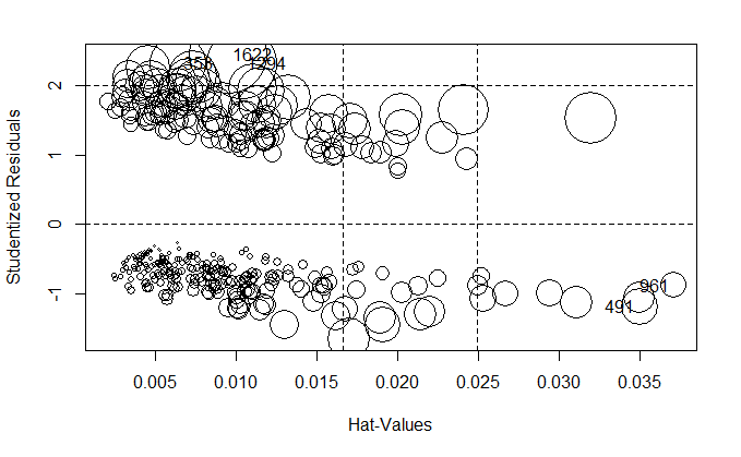
influencePlot(fit_reduced)
       StudRes         Hat       CookD
491  -1.184602 0.035017325 0.007381522
961  -0.878964 0.037140782 0.003674050
353   2.314756 0.006420789 0.016875451
1294  2.308549 0.010371085 0.026380976
1622  2.433243 0.009515004 0.032601703
解释模型参数
回归系数
coefficients(fit_reduced)
  (Intercept)           age  yearsmarried religiousness        rating
   1.93083017   -0.03527112    0.10062274   -0.32902386   -0.46136144
exp(coef(fit_reduced))
  (Intercept)           age  yearsmarried religiousness        rating
    6.8952321     0.9653437     1.1058594     0.7196258     0.6304248
系数的置信区间
confint(fit_reduced)
                    2.5 %       97.5 %
(Intercept)    0.75404303  3.150622807
age           -0.07006400 -0.001854759
yearsmarried   0.04388142  0.158562400
religiousness -0.50637196 -0.155156981
rating        -0.63741235 -0.288566411
exp(confint(fit_reduced))
                  2.5 %     97.5 %
(Intercept)   2.1255764 23.3506030
age           0.9323342  0.9981470
yearsmarried  1.0448584  1.1718250
religiousness 0.6026782  0.8562807
rating        0.5286586  0.7493370
评价预测变量对结果概率的影响
创建一个虚拟数据集,只有婚姻评分不同
test_data <- data.frame(
  rating=1:5,
  age=mean(Affairs$age),
  yearsmarried=mean(Affairs$yearsmarried),
  religiousness=mean(Affairs$religiousness)
)
test_data
  rating      age yearsmarried religiousness
1      1 32.48752     8.177696      3.116473
2      2 32.48752     8.177696      3.116473
3      3 32.48752     8.177696      3.116473
4      4 32.48752     8.177696      3.116473
5      5 32.48752     8.177696      3.116473
test_data$prob <- predict(
  fit_reduced,
  newdata=test_data,
  type="response"
)
test_data
  rating      age yearsmarried religiousness      prob
1      1 32.48752     8.177696      3.116473 0.5302296
2      2 32.48752     8.177696      3.116473 0.4157377
3      3 32.48752     8.177696      3.116473 0.3096712
4      4 32.48752     8.177696      3.116473 0.2204547
5      5 32.48752     8.177696      3.116473 0.1513079
年龄不同的虚拟数据集
test_data <- data.frame(
  rating=mean(Affairs$rating),
  age=seq(17, 57, 10),
  yearsmarried=mean(Affairs$yearsmarried),
  religiousness=mean(Affairs$religiousness)
)
test_data
   rating age yearsmarried religiousness
1 3.93178  17     8.177696      3.116473
2 3.93178  27     8.177696      3.116473
3 3.93178  37     8.177696      3.116473
4 3.93178  47     8.177696      3.116473
5 3.93178  57     8.177696      3.116473
test_data$prob <- predict(
  fit_reduced,
  newdata=test_data,
  type="response"
)
test_data
   rating age yearsmarried religiousness      prob
1 3.93178  17     8.177696      3.116473 0.3350834
2 3.93178  27     8.177696      3.116473 0.2615373
3 3.93178  37     8.177696      3.116473 0.1992953
4 3.93178  47     8.177696      3.116473 0.1488796
5 3.93178  57     8.177696      3.116473 0.1094738
过度离势
观测到的响应变量的方差大于期望的二项分布的方差。
检测方法1:二项分布模型的残差偏差除以残差自由度,如果比值比 1 大很多,可认为存在过度离势。
deviance(fit_reduced) / df.residual(fit_reduced)
[1] 1.03248
检测方法2:检验过度离势,需要拟合两次模型
fit <- glm(
  ynaffair ~ age + yearsmarried + religiousness + rating,
  data=Affairs,
  family=binomial()
)

fit_od <- glm(
  ynaffair ~ age + yearsmarried + religiousness + rating,
  data=Affairs,
  family=quasibinomial()
)

pchisq(
  summary(fit_od)$dispersion * fit$df.residual,
  fit$df.residual,
  lower=FALSE
)
[1] 0.340122
不显著,说明不存在过度离势
扩展
稳健 Logistic 回归
robust 包的 glmRob() 函数
多项分布回归
mlogit 包中的 mlogit() 函数
序数 Logistic 回归
rms 包中的 lrm() 函数
泊松回归
robust 包中的 breslow.dat 数据集
data(breslow.dat, package="robust")
head(breslow.dat)
   ID Y1 Y2 Y3 Y4 Base Age     Trt Ysum sumY Age10 Base4
1 104  5  3  3  3   11  31 placebo   14   14   3.1  2.75
2 106  3  5  3  3   11  30 placebo   14   14   3.0  2.75
3 107  2  4  0  5    6  25 placebo   11   11   2.5  1.50
4 114  4  4  1  4    8  36 placebo   13   13   3.6  2.00
5 116  7 18  9 21   66  22 placebo   55   55   2.2 16.50
6 118  5  2  8  7   27  29 placebo   22   22   2.9  6.75
summary(breslow.dat[c(6, 7, 8, 10)])
      Base             Age               Trt          sumY
 Min.   :  6.00   Min.   :18.00   placebo  :28   Min.   :  0.00
 1st Qu.: 12.00   1st Qu.:23.00   progabide:31   1st Qu.: 11.50
 Median : 22.00   Median :28.00                  Median : 16.00
 Mean   : 31.22   Mean   :28.34                  Mean   : 33.05
 3rd Qu.: 41.00   3rd Qu.:32.00                  3rd Qu.: 36.00
 Max.   :151.00   Max.   :42.00                  Max.   :302.00
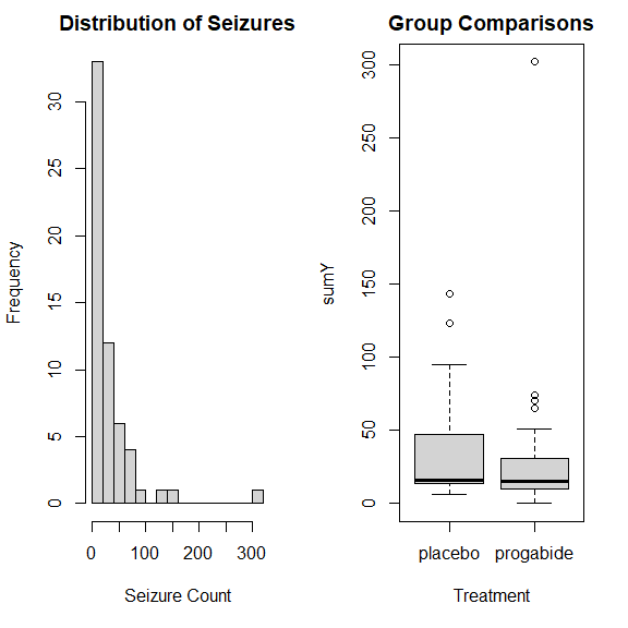
绘图分析
opar <- par(no.readonly=TRUE)
par(mfrow=c(1, 2))
with(
  breslow.dat,
  {
    hist(
      sumY,
      breaks=20,
      xlab="Seizure Count",
      main="Distribution of Seizures"
    )
    boxplot(
      sumY ~ Trt,
      xlab="Treatment",
      main="Group Comparisons"
    )
  }
)
par(opar)
泊松回归
fit <- glm(
  sumY ~ Base + Age + Trt,
  data=breslow.dat,
  family=poisson()
)
summary(fit)
Call:
glm(formula = sumY ~ Base + Age + Trt, family = poisson(), data = breslow.dat)

Deviance Residuals:
    Min       1Q   Median       3Q      Max
-6.0569  -2.0433  -0.9397   0.7929  11.0061

Coefficients:
               Estimate Std. Error z value Pr(>|z|)
(Intercept)   1.9488259  0.1356191  14.370  < 2e-16 ***
Base          0.0226517  0.0005093  44.476  < 2e-16 ***
Age           0.0227401  0.0040240   5.651 1.59e-08 ***
Trtprogabide -0.1527009  0.0478051  -3.194   0.0014 **
---
Signif. codes:  0 ‘***’ 0.001 ‘**’ 0.01 ‘*’ 0.05 ‘.’ 0.1 ‘ ’ 1

(Dispersion parameter for poisson family taken to be 1)

    Null deviance: 2122.73  on 58  degrees of freedom
Residual deviance:  559.44  on 55  degrees of freedom
AIC: 850.71

Number of Fisher Scoring iterations: 5
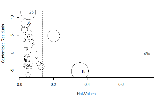
诊断图
influencePlot(fit)
解释模型参数
coef(fit)
 (Intercept)         Base          Age Trtprogabide
  1.94882593   0.02265174   0.02274013  -0.15270095
summary(fit)$coefficients
                Estimate   Std. Error   z value     Pr(>|z|)
(Intercept)   1.94882593 0.1356191170 14.369847 8.000803e-47
Base          0.02265174 0.0005093011 44.476125 0.000000e+00
Age           0.02274013 0.0040239969  5.651131 1.593953e-08
Trtprogabide -0.15270095 0.0478051047 -3.194239 1.401998e-03
exp(coef(fit))
 (Intercept)         Base          Age Trtprogabide
   7.0204403    1.0229102    1.0230007    0.8583864
过度离势
残差偏差 / 残差自由度
deviance(fit) / df.residual(fit)
[1] 10.1717
结果远大于 1,表明存在过度离势
qcc 包的 qcc.overdispersion.test() 函数检验泊松模型是否存在过度离势
library(qcc)
qcc.overdispersion.test(breslow.dat$sumY, type="poisson")
Overdispersion test Obs.Var/Theor.Var Statistic p-value
       poisson data          62.87013  3646.468       0
p 值小于 0.05,表明存在过度离势
类泊松方法
fit_od <- glm(
  sumY ~ Base + Age + Trt,
  data=breslow.dat,
  family=quasipoisson()
)
summary(fit_od)
Call:
glm(formula = sumY ~ Base + Age + Trt, family = quasipoisson(),
    data = breslow.dat)

Deviance Residuals:
    Min       1Q   Median       3Q      Max
-6.0569  -2.0433  -0.9397   0.7929  11.0061

Coefficients:
              Estimate Std. Error t value Pr(>|t|)
(Intercept)   1.948826   0.465091   4.190 0.000102 ***
Base          0.022652   0.001747  12.969  < 2e-16 ***
Age           0.022740   0.013800   1.648 0.105085
Trtprogabide -0.152701   0.163943  -0.931 0.355702
---
Signif. codes:  0 ‘***’ 0.001 ‘**’ 0.01 ‘*’ 0.05 ‘.’ 0.1 ‘ ’ 1

(Dispersion parameter for quasipoisson family taken to be 11.76075)

    Null deviance: 2122.73  on 58  degrees of freedom
Residual deviance:  559.44  on 55  degrees of freedom
AIC: NA

Number of Fisher Scoring iterations: 5
扩展
时间段变化的泊松回归
使用 glm() 中的 offset 选项
零膨胀的泊松回归
pscl 包中的 zeroinfl() 函数
稳健泊松回归
robust 包中的 glmRob() 函数
参考
https://github.com/perillaroc/r-in-action-study
R 语言实战
