R语言实战:重抽样与自助法
目录
本文内容来自《R 语言实战》(R in Action, 2nd),有部分修改
置换检验
置换检验,随机化检验,重随机化检验
精确检验 vs 蒙特卡洛模拟
使用 coin 包做置换检验
- 响应值与组的分配独立吗?
- 两个数值变量独立吗?
- 两个类别型别变量独立吗?
library(coin)
独立两样本和 K 样本检验
score <- c(
  40, 57, 45, 55, 58,
  57, 64, 55, 62, 65
)
treatment <- factor(
  c(rep("A", 5), rep("B", 5))
)
my_data <- data.frame(
  treatment, score
)
my_data
   treatment score
1          A    40
2          A    57
3          A    45
4          A    55
5          A    58
6          B    57
7          B    64
8          B    55
9          B    62
10         B    65
t 检验,结果显著
t.test(
  score ~ treatment,
  data=my_data,
  var.equal=TRUE
)
	Two Sample t-test

data:  score by treatment
t = -2.345, df = 8, p-value = 0.04705
alternative hypothesis: true difference in means is not equal to 0
95 percent confidence interval:
 -19.0405455  -0.1594545
sample estimates:
mean in group A mean in group B
           51.0            60.6
置换检验,结果不显著
oneway_test(
  score ~ treatment,
  data=my_data,
  distribution="exact"
)
	Exact Two-Sample Fisher-Pitman Permutation Test

data:  score by treatment (A, B)
Z = -1.9147, p-value = 0.07143
alternative hypothesis: true mu is not equal to 0
library(MASS)
UScrime <- transform(
  UScrime,
  So = factor(So)
)
head(UScrime)
    M So  Ed Po1 Po2  LF  M.F Pop  NW  U1 U2 GDP Ineq     Prob    Time    y
1 151  1  91  58  56 510  950  33 301 108 41 394  261 0.084602 26.2011  791
2 143  0 113 103  95 583 1012  13 102  96 36 557  194 0.029599 25.2999 1635
3 142  1  89  45  44 533  969  18 219  94 33 318  250 0.083401 24.3006  578
4 136  0 121 149 141 577  994 157  80 102 39 673  167 0.015801 29.9012 1969
5 141  0 121 109 101 591  985  18  30  91 20 578  174 0.041399 21.2998 1234
6 121  0 110 118 115 547  964  25  44  84 29 689  126 0.034201 20.9995  682
Wilcoxon 秩和检验
wilcox.test(
  Prob ~ So,
  data=UScrime,
)
	Wilcoxon rank sum exact test

data:  Prob by So
W = 81, p-value = 8.488e-05
alternative hypothesis: true location shift is not equal to 0
wilcox_test(
  Prob ~ So,
  data=UScrime,
  distribution="exact"
)
	Exact Wilcoxon-Mann-Whitney Test

data:  Prob by So (0, 1)
Z = -3.7493, p-value = 8.488e-05
alternative hypothesis: true mu is not equal to 0
近似 K 样本置换检验
library(multcomp)
head(cholesterol)
    trt response
1 1time   3.8612
2 1time  10.3868
3 1time   5.9059
4 1time   3.0609
5 1time   7.7204
6 1time   2.7139
set.seed(1234)
oneway_test(
  response ~ trt,
  data=cholesterol,
  distribution=approximate(nresample=9999)
)
	Approximative K-Sample Fisher-Pitman Permutation Test

data:  response by trt (1time, 2times, 4times, drugD, drugE)
chi-squared = 36.381, p-value < 1e-04
列联表中的独立性
chisq_test()、cmh_test()、lbl_test() 函数
library(vcd)
head(Arthritis)
  ID Treatment  Sex Age Improved
1 57   Treated Male  27     Some
2 46   Treated Male  29     None
3 77   Treated Male  30     None
4 17   Treated Male  32   Marked
5 36   Treated Male  46   Marked
6 23   Treated Male  58   Marked
Improved 是有序因子,进行线性趋势检验
set.seed(1234)
chisq_test(
  Treatment ~ Improved,
  data=Arthritis,
  distribution=approximate(nresample=9999)
)
	Approximative Linear-by-Linear Association Test

data:  Treatment by Improved (None < Some < Marked)
Z = -3.6075, p-value = 0.0006001
alternative hypothesis: two.sided
Arthritis_v2 <- transform(
  Arthritis,
  Improved=as.factor(as.numeric(Improved))
)
head(Arthritis_v2)
  ID Treatment  Sex Age Improved
1 57   Treated Male  27        2
2 46   Treated Male  29        1
3 77   Treated Male  30        1
4 17   Treated Male  32        3
5 36   Treated Male  46        3
6 23   Treated Male  58        3
Improved 是分类因子,进行卡方检验
set.seed(1234)
chisq_test(
  Treatment ~ Improved,
  data=Arthritis_v2,
  distribution=approximate(nresample=9999)
)
	Approximative Pearson Chi-Squared Test

data:  Treatment by Improved (1, 2, 3)
chi-squared = 13.055, p-value = 0.0018
数值变量间的独立性
spearman_test() 函数
states <- as.data.frame(state.x77)
head(states)
           Population Income Illiteracy Life Exp Murder HS Grad Frost
Alabama          3615   3624        2.1    69.05   15.1    41.3    20
Alaska            365   6315        1.5    69.31   11.3    66.7   152
Arizona          2212   4530        1.8    70.55    7.8    58.1    15
Arkansas         2110   3378        1.9    70.66   10.1    39.9    65
California      21198   5114        1.1    71.71   10.3    62.6    20
Colorado         2541   4884        0.7    72.06    6.8    63.9   166
             Area
Alabama     50708
Alaska     566432
Arizona    113417
Arkansas    51945
California 156361
Colorado   103766
set.seed(1234)
spearman_test(
  Illiteracy ~ Murder,
  data=states,
  distribution=approximate(nresample=9999)
)
	Approximative Spearman Correlation Test

data:  Illiteracy by Murder
Z = 4.7065, p-value < 1e-04
alternative hypothesis: true rho is not equal to 0
两样本和 K 样本相关性检验
两配对组的置换检验:wilcoxsign_test() 函数
多于两组:friedman_test() 函数
Wilcoxon 符号秩检验
wilcoxsign_test(
  U1 ~ U2,
  data=UScrime,
  distribution="exact"
)
	Exact Wilcoxon-Pratt Signed-Rank Test

data:  y by x (pos, neg)
	 stratified by block
Z = 5.9691, p-value = 1.421e-14
alternative hypothesis: true mu is not equal to 0
深入研究
independence_test() 函数
lmPerm 包的置换检验
线性模型的置换检验,比如 lmp() 和 aovp() 函数
library(lmPerm)
简单回归和多项式回归
set.seed(1234)
fit <- lmp(
  weight ~ height,
  data=women,
  perm="Prob"
)
[1] "Settings: unique SS : numeric variables centered"
summary(fit)
Call:
lmp(formula = weight ~ height, data = women, perm = "Prob")

Residuals:
    Min      1Q  Median      3Q     Max
-1.7333 -1.1333 -0.3833  0.7417  3.1167

Coefficients:
       Estimate Iter Pr(Prob)
height     3.45 5000   <2e-16 ***
---
Signif. codes:  0 ‘***’ 0.001 ‘**’ 0.01 ‘*’ 0.05 ‘.’ 0.1 ‘ ’ 1

Residual standard error: 1.525 on 13 degrees of freedom
Multiple R-Squared: 0.991,	Adjusted R-squared: 0.9903
F-statistic:  1433 on 1 and 13 DF,  p-value: 1.091e-14
二次方程
set.seed(1234)
fit <- lmp(
  weight ~ height + I(height^2),
  data=women,
  perm="Prob"
)
[1] "Settings: unique SS : numeric variables centered"
summary(fit)
Call:
lmp(formula = weight ~ height + I(height^2), data = women, perm = "Prob")

Residuals:
      Min        1Q    Median        3Q       Max
-0.509405 -0.296105 -0.009405  0.286151  0.597059

Coefficients:
            Estimate Iter Pr(Prob)
height      -7.34832 5000   <2e-16 ***
I(height^2)  0.08306 5000   <2e-16 ***
---
Signif. codes:  0 ‘***’ 0.001 ‘**’ 0.01 ‘*’ 0.05 ‘.’ 0.1 ‘ ’ 1

Residual standard error: 0.3841 on 12 degrees of freedom
Multiple R-Squared: 0.9995,	Adjusted R-squared: 0.9994
F-statistic: 1.139e+04 on 2 and 12 DF,  p-value: < 2.2e-16
多元回归
head(states)
           Population Income Illiteracy Life Exp Murder HS Grad Frost
Alabama          3615   3624        2.1    69.05   15.1    41.3    20
Alaska            365   6315        1.5    69.31   11.3    66.7   152
Arizona          2212   4530        1.8    70.55    7.8    58.1    15
Arkansas         2110   3378        1.9    70.66   10.1    39.9    65
California      21198   5114        1.1    71.71   10.3    62.6    20
Colorado         2541   4884        0.7    72.06    6.8    63.9   166
             Area
Alabama     50708
Alaska     566432
Arizona    113417
Arkansas    51945
California 156361
Colorado   103766
fit <- lmp(
  Murder ~ Population + Illiteracy + Income + Frost,
  data=states,
  perm="Prob"
)
[1] "Settings: unique SS : numeric variables centered"
summary(fit)
Call:
lmp(formula = Murder ~ Population + Illiteracy + Income + Frost,
    data = states, perm = "Prob")

Residuals:
     Min       1Q   Median       3Q      Max
-4.79597 -1.64946 -0.08112  1.48150  7.62104

Coefficients:
            Estimate Iter Pr(Prob)
Population 2.237e-04   51    1.000
Illiteracy 4.143e+00 5000   <2e-16 ***
Income     6.442e-05   51    0.961
Frost      5.813e-04   51    0.863
---
Signif. codes:  0 ‘***’ 0.001 ‘**’ 0.01 ‘*’ 0.05 ‘.’ 0.1 ‘ ’ 1

Residual standard error: 2.535 on 45 degrees of freedom
Multiple R-Squared: 0.567,	Adjusted R-squared: 0.5285
F-statistic: 14.73 on 4 and 45 DF,  p-value: 9.133e-08
fit <- lm(
  Murder ~ Population + Illiteracy + Income + Frost,
  data=states,
)
summary(fit)
Call:
lm(formula = Murder ~ Population + Illiteracy + Income + Frost,
    data = states)

Residuals:
    Min      1Q  Median      3Q     Max
-4.7960 -1.6495 -0.0811  1.4815  7.6210

Coefficients:
             Estimate Std. Error t value Pr(>|t|)
(Intercept) 1.235e+00  3.866e+00   0.319   0.7510
Population  2.237e-04  9.052e-05   2.471   0.0173 *
Illiteracy  4.143e+00  8.744e-01   4.738 2.19e-05 ***
Income      6.442e-05  6.837e-04   0.094   0.9253
Frost       5.813e-04  1.005e-02   0.058   0.9541
---
Signif. codes:  0 ‘***’ 0.001 ‘**’ 0.01 ‘*’ 0.05 ‘.’ 0.1 ‘ ’ 1

Residual standard error: 2.535 on 45 degrees of freedom
Multiple R-squared:  0.567,	Adjusted R-squared:  0.5285
F-statistic: 14.73 on 4 and 45 DF,  p-value: 9.133e-08
注意:在 lm() 中 Population 和 Illiteracy 均显著,而 lmp() 中仅 Illiteracy 显著
单因素方差分析和协方差分析
单因素方差分析的置换检验
set.seed(1234)
fit <- aovp(
  response ~ trt,
  data=cholesterol,
  perm="Prob"
)
[1] "Settings: unique SS "
anova(fit)
Analysis of Variance Table

Response: response
          Df R Sum Sq R Mean Sq Iter  Pr(Prob)
trt        4  1351.37    337.84 5000 < 2.2e-16 ***
Residuals 45   468.75     10.42
---
Signif. codes:  0 ‘***’ 0.001 ‘**’ 0.01 ‘*’ 0.05 ‘.’ 0.1 ‘ ’ 1
单因素协方差分析的置换检验
set.seed(1234)
fit <- aovp(
  weight ~ gesttime + dose,
  data=litter,
  perm="Prob"
)
[1] "Settings: unique SS : numeric variables centered"
anova(fit)
Analysis of Variance Table

Response: weight
          Df R Sum Sq R Mean Sq Iter Pr(Prob)
gesttime   1   161.49   161.493 5000   0.0006 ***
dose       3   137.12    45.708 5000   0.0392 *
Residuals 69  1151.27    16.685
---
Signif. codes:  0 ‘***’ 0.001 ‘**’ 0.01 ‘*’ 0.05 ‘.’ 0.1 ‘ ’ 1
双因素方差分析
set.seed(1234)
fit <- aovp(
  len ~ supp*dose,
  data=ToothGrowth,
  perm="Prob"
)
[1] "Settings: unique SS : numeric variables centered"
anova(fit)
Analysis of Variance Table

Response: len
          Df R Sum Sq R Mean Sq Iter Pr(Prob)
supp       1   205.35    205.35 5000  < 2e-16 ***
dose       1  2224.30   2224.30 5000  < 2e-16 ***
supp:dose  1    88.92     88.92 2032  0.04724 *
Residuals 56   933.63     16.67
---
Signif. codes:  0 ‘***’ 0.001 ‘**’ 0.01 ‘*’ 0.05 ‘.’ 0.1 ‘ ’ 1
置换检验点评
perm 包
corrperm 包
logregperm 包
glmperm 包
置换检验主要用于生成检验零假设的 p 值,有助于回答“效应是否存在”这样的问题。
自助法
从初始样本重复随机替换抽样,生成一个或一系列待检验统计量的经验分布。 无需假设一个特定的理论分布,便可生成统计量的置信区间,并能检验统计假设。
boot 包中的自助法
library("boot")
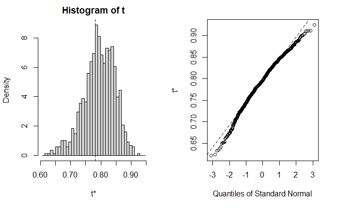
对单个统计量使用自助法
计算 R 平方的函数
rsq <- function(formula, data, indices) {
  d <- data[indices,]
  fit <- lm(formula, data=d)
  return (summary(fit)$r.square)
}
自助抽样
set.seed(1234)
results <- boot(
  data=mtcars,
  statistic=rsq,
  R=1000,
  formula=mpg ~ wt + disp
)
boot 对象可以输出
print(results)
ORDINARY NONPARAMETRIC BOOTSTRAP


Call:
boot(data = mtcars, statistic = rsq, R = 1000, formula = mpg ~
    wt + disp)


Bootstrap Statistics :
     original     bias    std. error
t1* 0.7809306 0.01379126  0.05113904
绘制结果
plot(results)
计算置信区间
ci_results <- boot.ci(
  results,
  type=c("perc", "bca")
)
ci_results
BOOTSTRAP CONFIDENCE INTERVAL CALCULATIONS
Based on 1000 bootstrap replicates

CALL :
boot.ci(boot.out = results, type = c("perc", "bca"))

Intervals :
Level     Percentile            BCa
95%   ( 0.6753,  0.8835 )   ( 0.6344,  0.8561 )
Calculations and Intervals on Original Scale
Some BCa intervals may be unstable
ci_results$percent
     conf
[1,] 0.95 25.03 975.98 0.6752993 0.8835035
ci_results$bca
     conf
[1,] 0.95 3.77 896.91 0.6343659 0.8560896
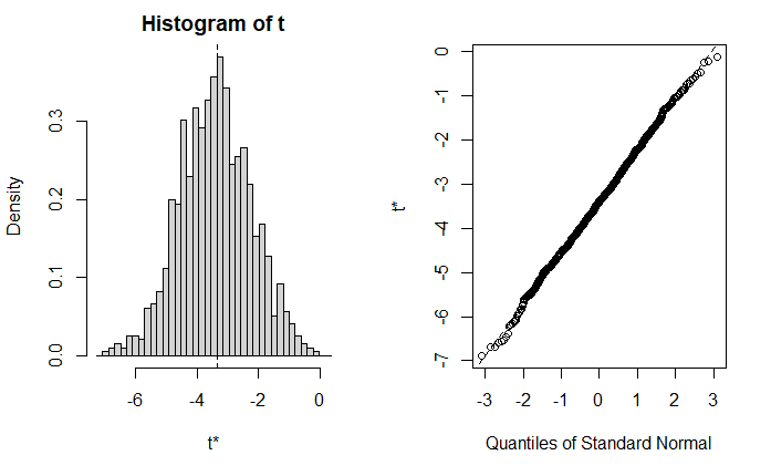
多个统计量的自助法
返回回归系数向量的函数
bs <- function(formula, data, indices) {
  d <- data[indices,]
  fit <- lm(formula, data=d)
  return(coef(fit))
}
自助抽样
set.seed(1234)
results <- boot(
  data=mtcars,
  statistic=bs,
  R=1000,
  formula=mpg ~ wt + disp
)
print(results)
ORDINARY NONPARAMETRIC BOOTSTRAP


Call:
boot(data = mtcars, statistic = bs, R = 1000, formula = mpg ~
    wt + disp)


Bootstrap Statistics :
       original        bias    std. error
t1* 34.96055404  4.715497e-02 2.546106756
t2* -3.35082533 -4.908125e-02 1.154800744
t3* -0.01772474  6.230927e-05 0.008518022
多个统计量使用索引
plot(
  results,
  index=2
)
置信区间
boot.ci(
  results,
  type="bca",
  index=2
)
BOOTSTRAP CONFIDENCE INTERVAL CALCULATIONS
Based on 1000 bootstrap replicates

CALL :
boot.ci(boot.out = results, type = "bca", index = 2)

Intervals :
Level       BCa
95%   (-5.477, -0.937 )
Calculations and Intervals on Original Scale
boot.ci(
  results,
  type="bca",
  index=3
)
BOOTSTRAP CONFIDENCE INTERVAL CALCULATIONS
Based on 1000 bootstrap replicates

CALL :
boot.ci(boot.out = results, type = "bca", index = 3)

Intervals :
Level       BCa
95%   (-0.0334, -0.0011 )
Calculations and Intervals on Original Scale
参考
https://github.com/perillaroc/r-in-action-study
R 语言实战
