ISLR习题:线性回归 - 线性模型的随机误差
目录
本文源自《统计学习导论:基于R语言应用》(ISLR) 第三章习题
向量 x,eps
set.seed(1)
x <- rnorm(100, 0, 1)
eps <- rnorm(100, 0, 0.25)
生成向量 y
y <- -1 + 0.25 * x + eps
其中
- beta_0 = -1
- beta_1 = 0.25
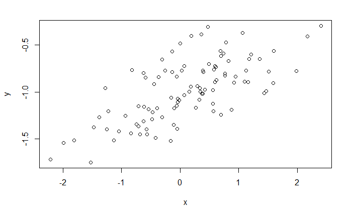
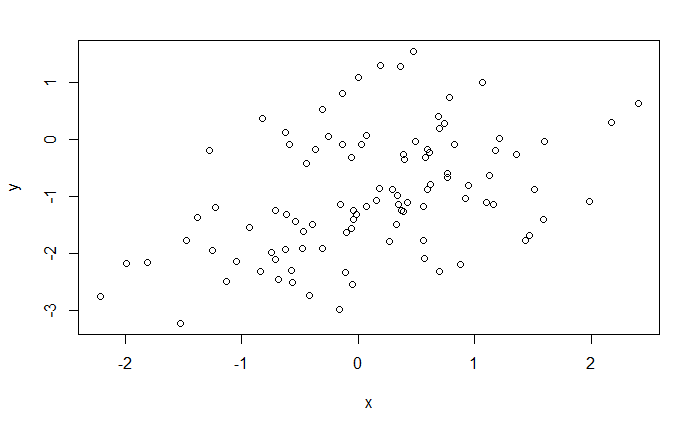
散点图
plot(x, y)
线性拟合
lm_fit_v1 <- lm(y ~ x)
summary(lm_fit_v1)
Call:
lm(formula = y ~ x)

Residuals:
     Min       1Q   Median       3Q      Max
-0.46921 -0.15344 -0.03487  0.13485  0.58654

Coefficients:
            Estimate Std. Error t value Pr(>|t|)
(Intercept) -1.00942    0.02425 -41.631  < 2e-16 ***
x            0.24973    0.02693   9.273 4.58e-15 ***
---
Signif. codes:  0 ‘***’ 0.001 ‘**’ 0.01 ‘*’ 0.05 ‘.’ 0.1 ‘ ’ 1

Residual standard error: 0.2407 on 98 degrees of freedom
Multiple R-squared:  0.4674,	Adjusted R-squared:  0.4619
F-statistic: 85.99 on 1 and 98 DF,  p-value: 4.583e-15
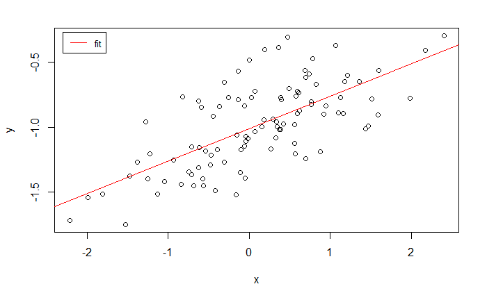
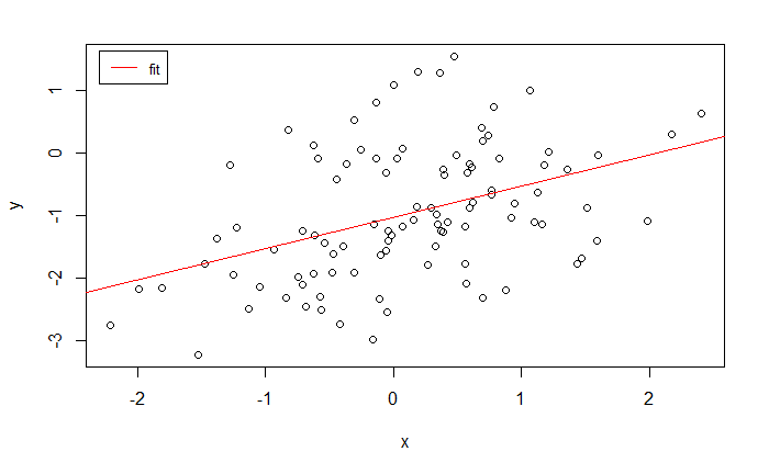
拟合得到的系数与真实值比较接近
拟合线
plot(x, y)
abline(lm_fit_v1, col="red")
legend(
  "topleft",
  inset=.02,
  legend=c("fit"),
  col=c("red"),
  lty=1:2,
  cex=0.8
)
多项式拟合
lm_fit_v2 <- lm(y ~ x + I(x^2))
summary(lm_fit_v2)
Call:
lm(formula = y ~ x + I(x^2))

Residuals:
    Min      1Q  Median      3Q     Max
-0.4913 -0.1563 -0.0322  0.1451  0.5675

Coefficients:
            Estimate Std. Error t value Pr(>|t|)
(Intercept) -0.98582    0.02941 -33.516  < 2e-16 ***
x            0.25429    0.02700   9.420  2.4e-15 ***
I(x^2)      -0.02973    0.02119  -1.403    0.164
---
Signif. codes:  0 ‘***’ 0.001 ‘**’ 0.01 ‘*’ 0.05 ‘.’ 0.1 ‘ ’ 1

Residual standard error: 0.2395 on 97 degrees of freedom
Multiple R-squared:  0.4779,	Adjusted R-squared:  0.4672
F-statistic:  44.4 on 2 and 97 DF,  p-value: 2.038e-14
虽然残差标准误有所降低,但 x^2 项的 p 值太大,没有显著性。
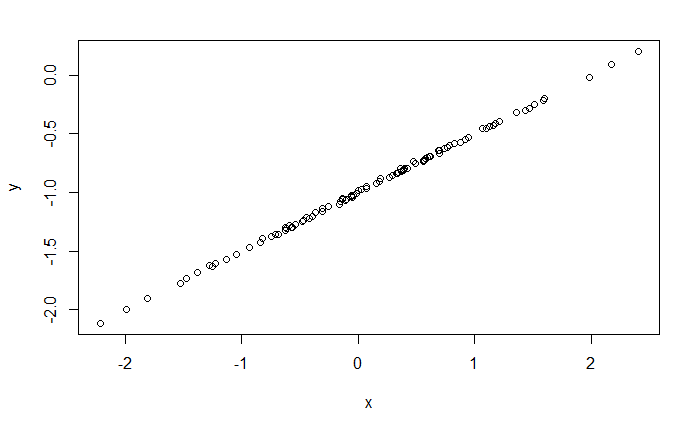
低噪声
set.seed(1)
x <- rnorm(100)
eps <- rnorm(100, 0, 0.01)
y <- -1 + 0.5 * x + eps
plot(x, y)
lm_fit_v3 <- lm(y ~ x)
summary(lm_fit_v3)
Call:
lm(formula = y ~ x)
Residuals:
Min 1Q Median 3Q Max
-0.018768 -0.006138 -0.001395 0.005394 0.023462
Coefficients:
Estimate Std. Error t value Pr(>|t|)
(Intercept) -1.0003769 0.0009699 -1031.5 <2e-16 ***
x 0.4999894 0.0010773 464.1 <2e-16 ***
---
Signif. codes: 0 ‘***’ 0.001 ‘**’ 0.01 ‘*’ 0.05 ‘.’ 0.1 ‘ ’ 1
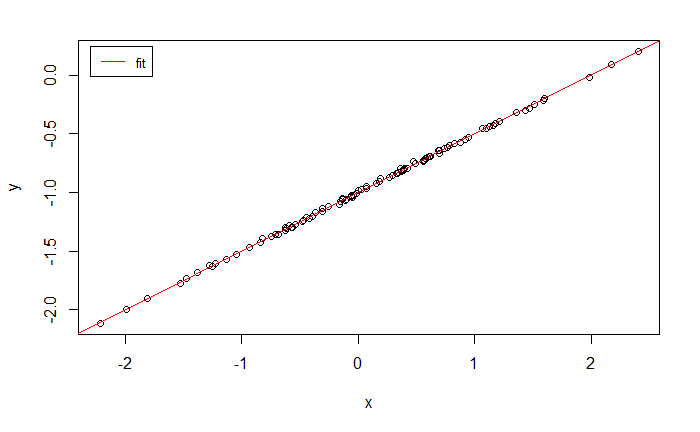
Residual standard error: 0.009628 on 98 degrees of freedom
Multiple R-squared: 0.9995, Adjusted R-squared: 0.9995
F-statistic: 2.154e+05 on 1 and 98 DF, p-value: < 2.2e-16
plot(x, y)
abline(lm_fit_v3, col="red")
legend(
  "topleft",
  inset=.02,
  legend=c("fit"),
  col=c("red"),
  lty=1:2,
  cex=0.8
)
高噪声
set.seed(1)
x <- rnorm(100)
eps <- rnorm(100, 0, 1.0)
y <- -1 + 0.5 * x + eps
plot(x, y)
lm_fit_v4 <- lm(y ~ x)
summary(lm_fit_v4)
plot(x, y)
abline(lm_fit_v4, col="red")
legend("topleft", inset=.02, legend=c("fit"), col=c("red"), lty=1:2, cex=0.8)
对比
求置信区间
原始数据集
confint(lm_fit_v1)
                 2.5 %     97.5 %
(Intercept) -1.0575402 -0.9613061
x            0.1962897  0.3031801
低噪声数据集
confint(lm_fit_v3)
                 2.5 %     97.5 %
(Intercept) -1.0023016 -0.9984522
x            0.4978516  0.5021272
高噪声数据集
confint(lm_fit_v4)
                 2.5 %     97.5 %
(Intercept) -1.2301607 -0.8452245
x            0.2851588  0.7127204
置信区间随着噪声的增大而增大
参考
https://github.com/perillaroc/islr-study
ISLR实验系列文章
线性回归
分类
重抽样方法
线性模型选择与正则化
