ISLR习题:线性回归 - 共线性问题
目录
本文源自《统计学习导论:基于R语言应用》(ISLR) 第三章习题
创建一组有共线性关系的数据集
set.seed(1)
x1 <- runif(100)
x2 <- 0.5 + x1 + rnorm(100) / 10
y <- 2 + 2 * x1 + 0.3 * x2 + rnorm(100)
$$ y = 2 + 2x_1 + 0.3x_2 $$
相关性
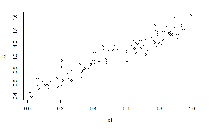
cor(x1, x2)
[1] 0.9469723
plot(x1, x2)
拟合
lm_fit_v1 <- lm(y ~ x1 + x2)
summary(lm_fit_v1)
Call:
lm(formula = y ~ x1 + x2)

Residuals:
    Min      1Q  Median      3Q     Max
-2.8311 -0.7273 -0.0537  0.6338  2.3359

Coefficients:
            Estimate Std. Error t value Pr(>|t|)
(Intercept)   1.7757     0.5933   2.993  0.00351 **
x1            1.0847     1.2346   0.879  0.38179
x2            1.0097     1.1337   0.891  0.37536
---
Signif. codes:  0 ‘***’ 0.001 ‘**’ 0.01 ‘*’ 0.05 ‘.’ 0.1 ‘ ’ 1

Residual standard error: 1.056 on 97 degrees of freedom
Multiple R-squared:  0.2333,	Adjusted R-squared:  0.2175
F-statistic: 14.76 on 2 and 97 DF,  p-value: 2.54e-06
预测的 beta_1 和 beta_2 与真实值相差过大
x1 和 x2 系数的 p 值过小,不能拒绝零假设
单变量拟合
y 对 x1
lm_fit_x1 <- lm(y ~ x1)
summary(lm_fit_x1)
Call:
lm(formula = y ~ x1)

Residuals:
     Min       1Q   Median       3Q      Max
-2.89495 -0.66874 -0.07785  0.59221  2.45560

Coefficients:
            Estimate Std. Error t value Pr(>|t|)
(Intercept)   2.2624     0.2307   9.805 3.21e-16 ***
x1            2.1259     0.3963   5.365 5.42e-07 ***
---
Signif. codes:  0 ‘***’ 0.001 ‘**’ 0.01 ‘*’ 0.05 ‘.’ 0.1 ‘ ’ 1

Residual standard error: 1.055 on 98 degrees of freedom
Multiple R-squared:  0.227,	Adjusted R-squared:  0.2191
F-statistic: 28.78 on 1 and 98 DF,  p-value: 5.42e-07
p 值几乎为 0,可以拒绝零假设
y 对 x2
lm_fit_x2 <- lm(y ~ x2)
summary(lm_fit_x2)
Call:
lm(formula = y ~ x2)

Residuals:
     Min       1Q   Median       3Q      Max
-2.74970 -0.68815 -0.03074  0.66090  2.34837

Coefficients:
            Estimate Std. Error t value Pr(>|t|)
(Intercept)   1.3789     0.3845   3.587 0.000525 ***
x2            1.9529     0.3639   5.367 5.36e-07 ***
---
Signif. codes:  0 ‘***’ 0.001 ‘**’ 0.01 ‘*’ 0.05 ‘.’ 0.1 ‘ ’ 1

Residual standard error: 1.055 on 98 degrees of freedom
Multiple R-squared:  0.2272,	Adjusted R-squared:  0.2193
F-statistic: 28.81 on 1 and 98 DF,  p-value: 5.361e-07
p 值几乎为 0,可以拒绝零假设
错误观测
x1 <- c(x1, 0.1)
x2 <- c(x2, 0.8)
y <- c(y, 6)
多变量
y 对 x1 和 x2
lm_fit_v2 <- lm(y ~ x1 + x2)
summary(lm_fit_v2)
Call:
lm(formula = y ~ x1 + x2)

Residuals:
     Min       1Q   Median       3Q      Max
-2.77906 -0.72031 -0.05796  0.62800  3.04112

Coefficients:
            Estimate Std. Error t value Pr(>|t|)
(Intercept)   1.5360     0.6115   2.512   0.0136 *
x1            0.1292     1.2407   0.104   0.9173
x2            1.7624     1.1500   1.532   0.1286
---
Signif. codes:  0 ‘***’ 0.001 ‘**’ 0.01 ‘*’ 0.05 ‘.’ 0.1 ‘ ’ 1

Residual standard error: 1.099 on 98 degrees of freedom
Multiple R-squared:  0.201,	Adjusted R-squared:  0.1847
F-statistic: 12.32 on 2 and 98 DF,  p-value: 1.682e-05
plot(lm_fit_v2)

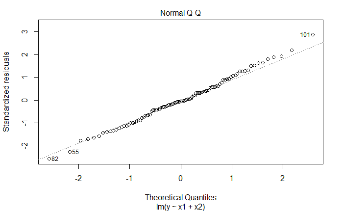
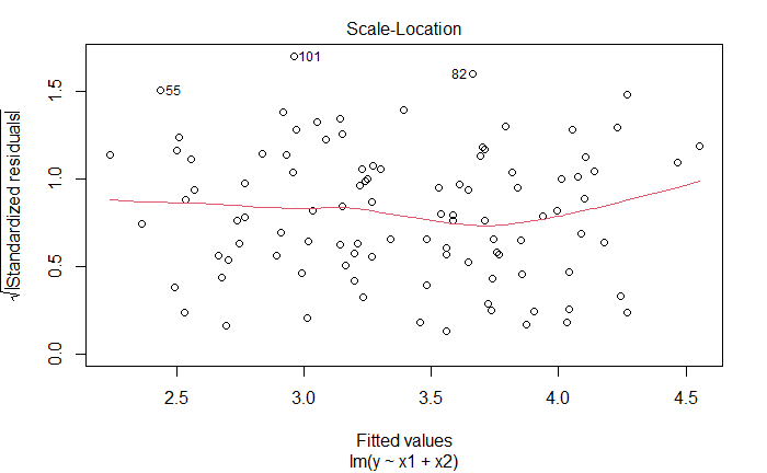
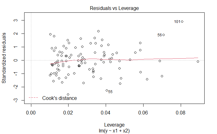
新增观测是离群点,也是高杠杆点
单变量
y 对 x1
lm_fit_x1_v2 <- lm(y ~ x1)
summary(lm_fit_x1_v2)
Call:
lm(formula = y ~ x1)

Residuals:
    Min      1Q  Median      3Q     Max
-2.8899 -0.6553 -0.0917  0.5679  3.4070

Coefficients:
            Estimate Std. Error t value Pr(>|t|)
(Intercept)   2.4005     0.2378   10.09  < 2e-16 ***
x1            1.9251     0.4104    4.69 8.74e-06 ***
---
Signif. codes:  0 ‘***’ 0.001 ‘**’ 0.01 ‘*’ 0.05 ‘.’ 0.1 ‘ ’ 1

Residual standard error: 1.106 on 99 degrees of freedom
Multiple R-squared:  0.1818,	Adjusted R-squared:  0.1736
F-statistic:    22 on 1 and 99 DF,  p-value: 8.744e-06
plot(lm_fit_x1_v2)
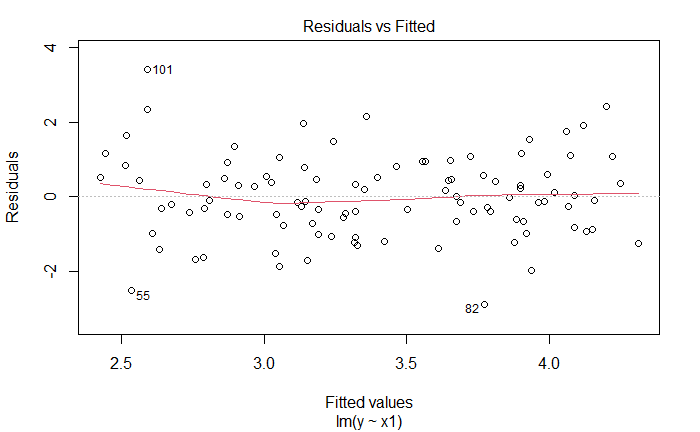
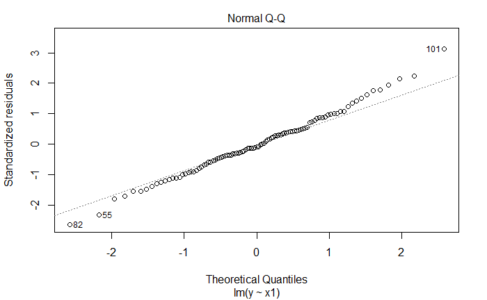
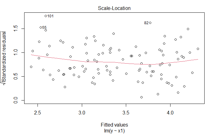
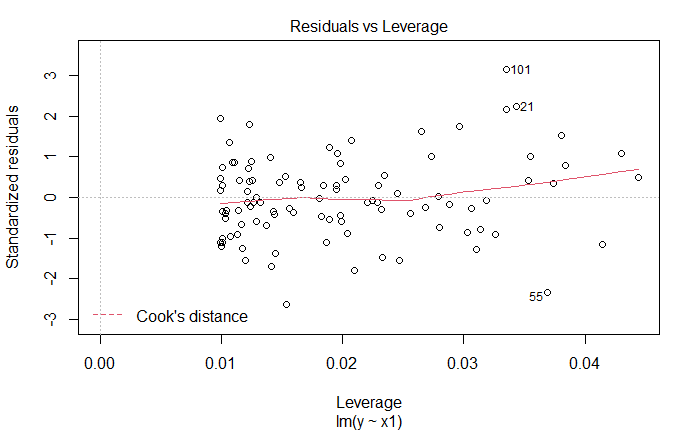
新增观测是离群点,也是高杠杆点
y 对 x2
lm_fit_x2_v2 <- lm(y ~ x2)
summary(lm_fit_x2_v2)
Call:
lm(formula = y ~ x2)

Residuals:
     Min       1Q   Median       3Q      Max
-2.76917 -0.70920 -0.04555  0.64028  3.01186

Coefficients:
            Estimate Std. Error t value Pr(>|t|)
(Intercept)   1.4877     0.3964   3.753 0.000295 ***
x2            1.8755     0.3760   4.989  2.6e-06 ***
---
Signif. codes:  0 ‘***’ 0.001 ‘**’ 0.01 ‘*’ 0.05 ‘.’ 0.1 ‘ ’ 1

Residual standard error: 1.093 on 99 degrees of freedom
Multiple R-squared:  0.2009,	Adjusted R-squared:  0.1928
F-statistic: 24.89 on 1 and 99 DF,  p-value: 2.601e-06
plot(lm_fit_x2_v2)
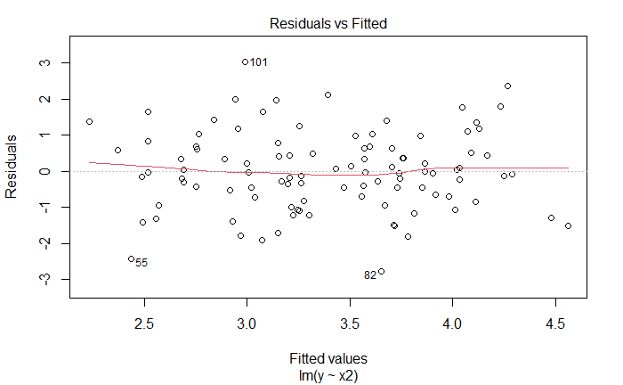
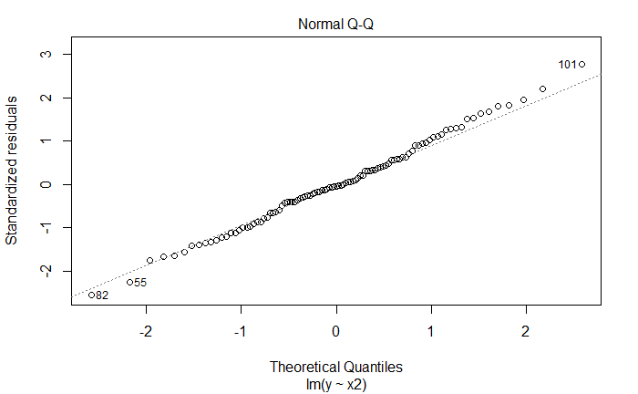
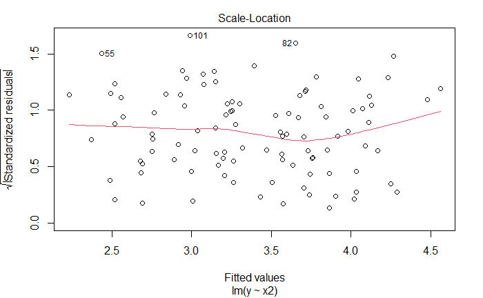
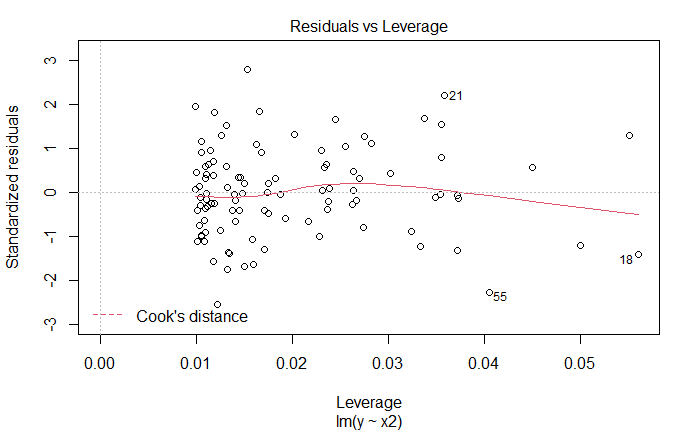
新增观测是离群点,但不是高杠杆点
参考
https://github.com/perillaroc/islr-study
ISLR实验系列文章
线性回归
分类
重抽样方法
线性模型选择与正则化
