ISLR习题：线性回归 - Carseats数据集

January 13, 2021 (最后修改: November 08, 2024)

本文源自《统计学习导论：基于R语言应用》(ISLR) 第三章习题

library(ISLR)

Carseats 数据集

head(Carseats)

  Sales CompPrice Income Advertising Population Price ShelveLoc Age Education Urban  US
1  9.50       138     73          11        276   120       Bad  42        17   Yes Yes
2 11.22       111     48          16        260    83      Good  65        10   Yes Yes
3 10.06       113     35          10        269    80    Medium  59        12   Yes Yes
4  7.40       117    100           4        466    97    Medium  55        14   Yes Yes
5  4.15       141     64           3        340   128       Bad  38        13   Yes  No
6 10.81       124    113          13        501    72       Bad  78        16    No Yes

nrow(Carseats)

[1] 400

多元回归

lm_fit_multi <- lm(
  Sales ~ Price + Urban + US,
  data=Carseats
)
summary(lm_fit_multi)

Call:
lm(formula = Sales ~ Price + Urban + US, data = Carseats)

Residuals:
    Min      1Q  Median      3Q     Max 
-6.9206 -1.6220 -0.0564  1.5786  7.0581 

Coefficients:
             Estimate Std. Error t value Pr(>|t|)    
(Intercept) 13.043469   0.651012  20.036  < 2e-16 ***
Price       -0.054459   0.005242 -10.389  < 2e-16 ***
UrbanYes    -0.021916   0.271650  -0.081    0.936    
USYes        1.200573   0.259042   4.635 4.86e-06 ***
---
Signif. codes:  0 ‘***’ 0.001 ‘**’ 0.01 ‘*’ 0.05 ‘.’ 0.1 ‘ ’ 1

Residual standard error: 2.472 on 396 degrees of freedom
Multiple R-squared:  0.2393,	Adjusted R-squared:  0.2335 
F-statistic: 41.52 on 3 and 396 DF,  p-value: < 2.2e-16

解释系数

Price 是数值量，与 Sales 呈负相关。

Urban 是定性变量，UrbanYes 表示是 Urban 为 Yes。

US 是定性变量，USYes 表示 US 为 Yes。

方程形式

把模型写成方程形式

$$ \begin{equation} \begin{aligned} sales &= \beta_0 + \beta_1p + \beta_2x_{i1} + \beta_3x_{i2} \\ &= \beta_0 + \beta_1p + \left\{\begin{matrix} \beta_2 + \beta_3 & \textit{Urban and US} \\ \beta_2 & \textit{Urban only} \\ \beta_3 & \textit{US only} \\ 0 & none \end{matrix} \right. \end{aligned} \end{equation} $$

零假设

Price 和 USYes 的 p 值几乎为 0，可以拒绝零假设。

新模型

UrbanYes 没有显著性，去掉该变量重新拟合模型

lm_fit_multi_new <- lm(
  Sales ~ Price + US,
  data=Carseats
)
summary(lm_fit_multi_new)

Call:
lm(formula = Sales ~ Price + US, data = Carseats)

Residuals:
    Min      1Q  Median      3Q     Max 
-6.9269 -1.6286 -0.0574  1.5766  7.0515 

Coefficients:
            Estimate Std. Error t value Pr(>|t|)    
(Intercept) 13.03079    0.63098  20.652  < 2e-16 ***
Price       -0.05448    0.00523 -10.416  < 2e-16 ***
USYes        1.19964    0.25846   4.641 4.71e-06 ***
---
Signif. codes:  0 ‘***’ 0.001 ‘**’ 0.01 ‘*’ 0.05 ‘.’ 0.1 ‘ ’ 1

Residual standard error: 2.469 on 397 degrees of freedom
Multiple R-squared:  0.2393,	Adjusted R-squared:  0.2354 
F-statistic: 62.43 on 2 and 397 DF,  p-value: < 2.2e-16

模型拟合效果对比

模型	Residual standard error	Multiple R-squared	Adjusted R-squared
model 1	2.472	0.2393	0.2335
model 2	2.469	0.2393	0.2354

model 2 的残差标准误和R方统计量均优于 model 1，但效果改善不是很明显。

系数的置信区间

confint(lm_fit_multi_new)

                  2.5 %      97.5 %
(Intercept) 11.79032020 14.27126531
Price       -0.06475984 -0.04419543
USYes        0.69151957  1.70776632

诊断图

plot(lm_fit_multi_new)

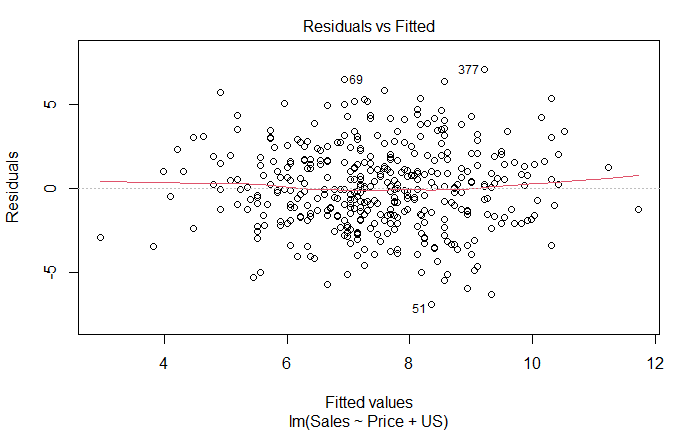
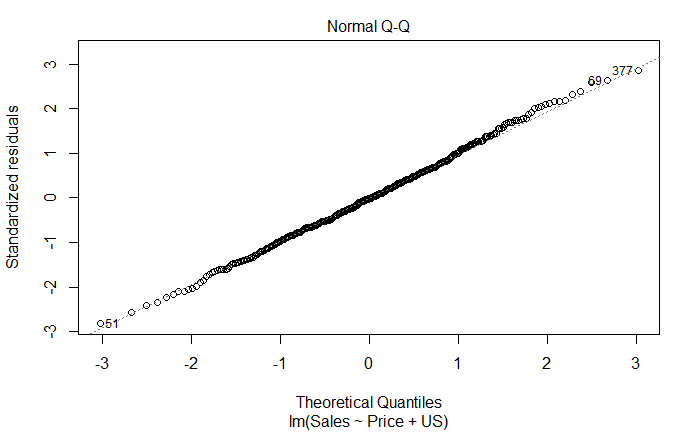
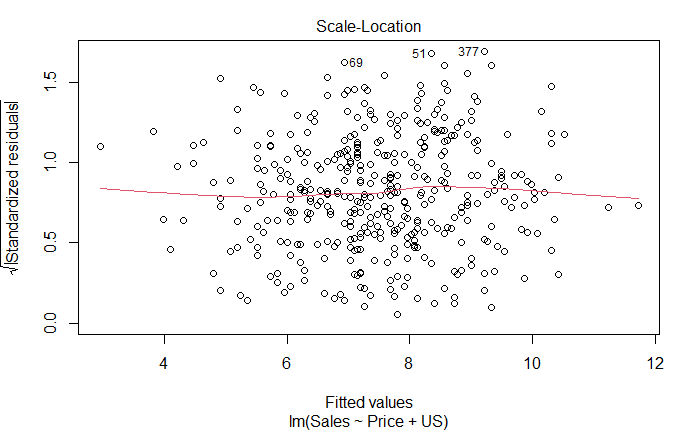
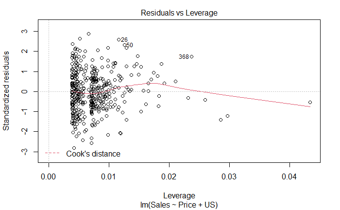
从残差图可以看到，模型有离群点

从杠杆统计量和学生化残差图中可以看到，有高杠杆点。

参考

https://github.com/perillaroc/islr-study

ISLR实验系列文章

线性回归

分类

重抽样方法

交叉验证法和自助法

线性模型选择与正则化