ISLR习题:线性回归 - Auto数据集
目录
本文源自《统计学习导论:基于R语言应用》(ISLR) 第三章习题
library(ISLR)
head(Auto)
  mpg cylinders displacement horsepower weight acceleration year origin                      name
1  18         8          307        130   3504         12.0   70      1 chevrolet chevelle malibu
2  15         8          350        165   3693         11.5   70      1         buick skylark 320
3  18         8          318        150   3436         11.0   70      1        plymouth satellite
4  16         8          304        150   3433         12.0   70      1             amc rebel sst
5  17         8          302        140   3449         10.5   70      1               ford torino
6  15         8          429        198   4341         10.0   70      1          ford galaxie 500
attach(Auto)
简单线性回归
mpg (油耗) 是响应变量,horsepower (马力) 是预测变量
创建模型
lm_fit = lm(horsepower ~ mpg)
lm_fit
Call:
lm(formula = horsepower ~ mpg)

Coefficients:
(Intercept)          mpg
    194.476       -3.839
查看模型
summary(lm_fit)
Call:
lm(formula = horsepower ~ mpg)

Residuals:
    Min      1Q  Median      3Q     Max
-64.892 -15.716  -2.094  13.108  96.947

Coefficients:
            Estimate Std. Error t value Pr(>|t|)
(Intercept) 194.4756     3.8732   50.21   <2e-16 ***
mpg          -3.8389     0.1568  -24.49   <2e-16 ***
---
Signif. codes:  0 ‘***’ 0.001 ‘**’ 0.01 ‘*’ 0.05 ‘.’ 0.1 ‘ ’ 1

Residual standard error: 24.19 on 390 degrees of freedom
Multiple R-squared:  0.6059,	Adjusted R-squared:  0.6049
F-statistic: 599.7 on 1 and 390 DF,  p-value: < 2.2e-16
简要分析
预测变量与响应变量之间有关联
Pr 值接近 0,两者有很强的相关性
mpg 的系数为负,两者负相关
预测
mpg 为 98 时,计算预测值
predict(lm_fit, data.frame(mpg=c(98)))
        1
-181.7354
计算置信区间
predict(
  lm_fit,
  data.frame(mpg=c(98)),
  interval="confidence"
)
        fit       lwr       upr
1 -181.7354 -204.8381 -158.6327
计算预测区间
predict(
  lm_fit,
  data.frame(mpg=c(98)),
  interval="prediction"
)
        fit       lwr       upr
1 -181.7354 -234.6145 -128.8562
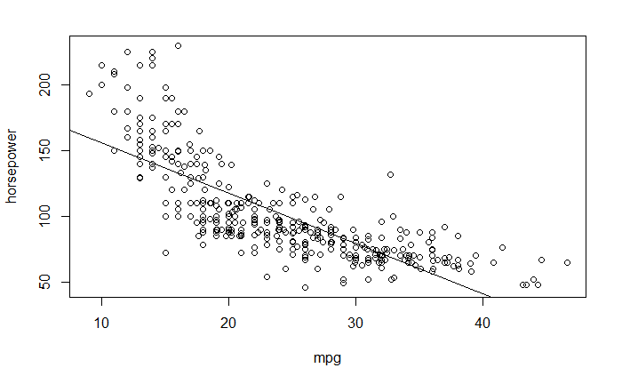
关系图
plot(mpg, horsepower)
abline(lm_fit)
诊断图
使用 plot() 生成最小二乘回归拟合的诊断图
plot(lm_fit)
残差图
Residuals vs Fitted
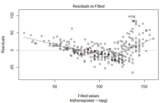
图中有明显的规律,残差值与估计值有关,说明线性模型的某些方面可能存在问题。
正态 QQ 图
Normal Q-Q
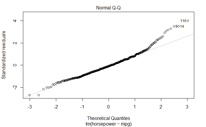
如果满足正态性假设,残差也应该是一个均值为 0 的正态分布,图上的点应该落在呈 45 度角的直线上。
Scale-Location
与第一幅图类似,显示标准化残差与估计值的关系。
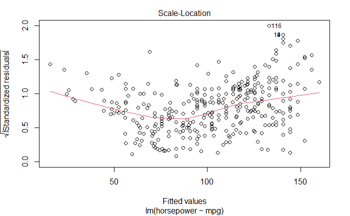
图中有比较明显的趋势,同样说明模型有问题。
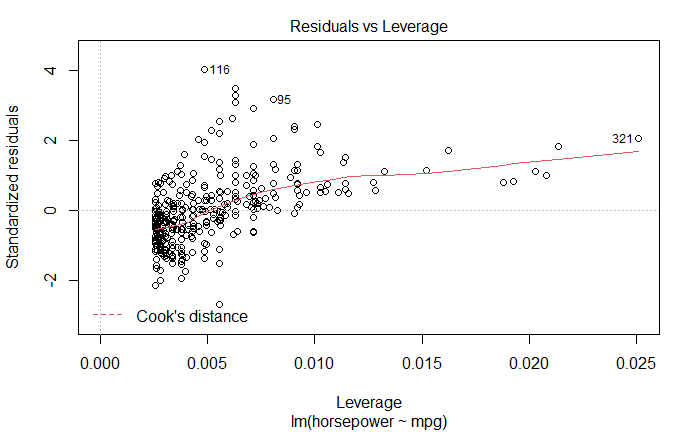
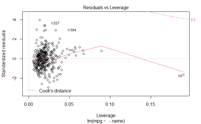
Residuals vs Leverage
杠杆统计量与学生化残差的关系图,用于查看离群点和高杠杆点。
多元线性回归
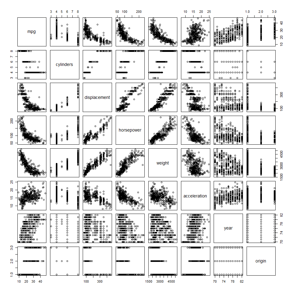
散点矩阵图
plot(Auto[, -c(9)])
相关系数矩阵
data.frame(cor(Auto[,-9]))
                    mpg  cylinders displacement horsepower     weight acceleration       year     origin
mpg           1.0000000 -0.7776175   -0.8051269 -0.7784268 -0.8322442    0.4233285  0.5805410  0.5652088
cylinders    -0.7776175  1.0000000    0.9508233  0.8429834  0.8975273   -0.5046834 -0.3456474 -0.5689316
displacement -0.8051269  0.9508233    1.0000000  0.8972570  0.9329944   -0.5438005 -0.3698552 -0.6145351
horsepower   -0.7784268  0.8429834    0.8972570  1.0000000  0.8645377   -0.6891955 -0.4163615 -0.4551715
weight       -0.8322442  0.8975273    0.9329944  0.8645377  1.0000000   -0.4168392 -0.3091199 -0.5850054
acceleration  0.4233285 -0.5046834   -0.5438005 -0.6891955 -0.4168392    1.0000000  0.2903161  0.2127458
year          0.5805410 -0.3456474   -0.3698552 -0.4163615 -0.3091199    0.2903161  1.0000000  0.1815277
origin        0.5652088 -0.5689316   -0.6145351 -0.4551715 -0.5850054    0.2127458  0.1815277  1.0000000
多元线性回归
lm_fit_multi <- lm(mpg~.-name, data=Auto)
summary(lm_fit_multi)
Call:
lm(formula = mpg ~ . - name, data = Auto)

Residuals:
    Min      1Q  Median      3Q     Max
-9.5903 -2.1565 -0.1169  1.8690 13.0604

Coefficients:
               Estimate Std. Error t value Pr(>|t|)
(Intercept)  -17.218435   4.644294  -3.707  0.00024 ***
cylinders     -0.493376   0.323282  -1.526  0.12780
displacement   0.019896   0.007515   2.647  0.00844 **
horsepower    -0.016951   0.013787  -1.230  0.21963
weight        -0.006474   0.000652  -9.929  < 2e-16 ***
acceleration   0.080576   0.098845   0.815  0.41548
year           0.750773   0.050973  14.729  < 2e-16 ***
origin         1.426141   0.278136   5.127 4.67e-07 ***
---
Signif. codes:  0 ‘***’ 0.001 ‘**’ 0.01 ‘*’ 0.05 ‘.’ 0.1 ‘ ’ 1

Residual standard error: 3.328 on 384 degrees of freedom
Multiple R-squared:  0.8215,	Adjusted R-squared:  0.8182
F-statistic: 252.4 on 7 and 384 DF,  p-value: < 2.2e-16
- 预测变量和响应变量之间是否有关系?
F 统计量为 252.4,远大于 1,且 F 统计量的 p 值几乎为零。 说明至少一个预测变量与响应变量有关系。
- 哪个预测变量与响应变量在统计上具有显著关系?
从预测变量的 p 值看,displacement,weight,year 和 origin 的 p 值较小,与响应变量具有显著关系。
- year 车龄变量的系数说明什么?
year 的系数为正值,说明随着车龄增长,油耗会增加。
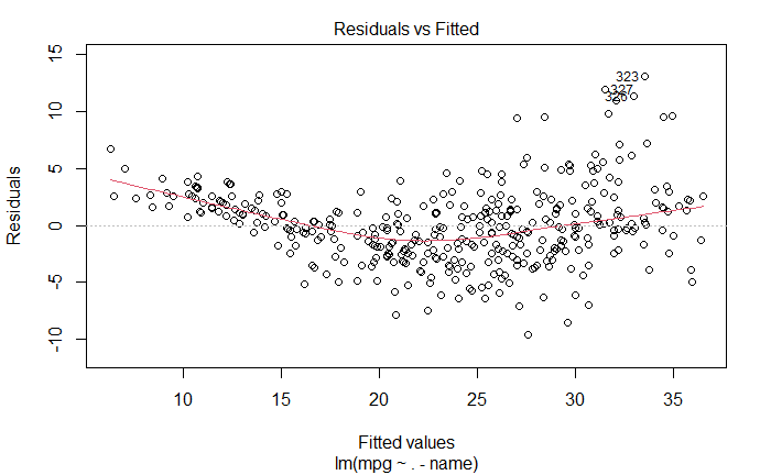
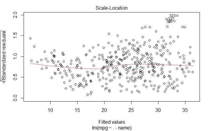
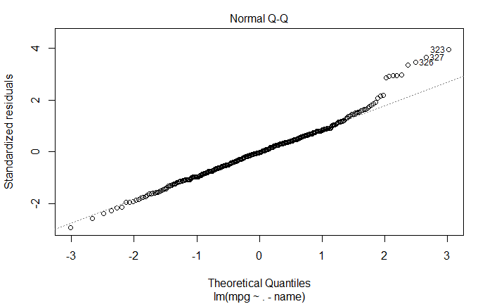
诊断图
plot(lm_fit_multi)
- 残差图是否有异常大的离群点?
有异常点,图中已标明
- 杠杆图是否识别出了有异常高杠杆作用的点么?
已标明,第 14 个样本
- Normal Q-Q
残差不按正态分布
交互作用
lm_fit_inter <- lm(
  mpg ~ .-name + cylinders * horsepower,
  data=Auto
)
summary(lm_fit_inter)
Call:
lm(formula = mpg ~ . - name + cylinders * horsepower, data = Auto)

Residuals:
    Min      1Q  Median      3Q     Max
-9.2399 -1.6871 -0.0511  1.2858 11.9380

Coefficients:
                       Estimate Std. Error t value Pr(>|t|)
(Intercept)          11.7025260  4.9115648   2.383 0.017676 *
cylinders            -4.3060695  0.4580950  -9.400  < 2e-16 ***
displacement         -0.0013925  0.0069110  -0.201 0.840426
horsepower           -0.3156601  0.0306339 -10.304  < 2e-16 ***
weight               -0.0038948  0.0006231  -6.250 1.09e-09 ***
acceleration         -0.1703028  0.0901427  -1.889 0.059612 .
year                  0.7393193  0.0448736  16.476  < 2e-16 ***
origin                0.9031644  0.2496880   3.617 0.000338 ***
cylinders:horsepower  0.0402008  0.0037856  10.619  < 2e-16 ***
---
Signif. codes:  0 ‘***’ 0.001 ‘**’ 0.01 ‘*’ 0.05 ‘.’ 0.1 ‘ ’ 1

Residual standard error: 2.929 on 383 degrees of freedom
Multiple R-squared:  0.8621,	Adjusted R-squared:  0.8592
F-statistic: 299.3 on 8 and 383 DF,  p-value: < 2.2e-16
存在统计显著的交互项,不过系数较小。
非线性变换
lm_fit_non_linear <- lm(
  mpg ~ .-name + log(horsepower),
  data=Auto
)
summary(lm_fit_non_linear)
Call:
lm(formula = mpg ~ . - name + log(horsepower), data = Auto)

Residuals:
    Min      1Q  Median      3Q     Max
-8.5777 -1.6623 -0.1213  1.4913 12.0230

Coefficients:
                  Estimate Std. Error t value Pr(>|t|)
(Intercept)      8.674e+01  1.106e+01   7.839 4.54e-14 ***
cylinders       -5.530e-02  2.907e-01  -0.190 0.849230
displacement    -4.607e-03  7.108e-03  -0.648 0.517291
horsepower       1.764e-01  2.269e-02   7.775 7.05e-14 ***
weight          -3.366e-03  6.561e-04  -5.130 4.62e-07 ***
acceleration    -3.277e-01  9.670e-02  -3.388 0.000776 ***
year             7.421e-01  4.534e-02  16.368  < 2e-16 ***
origin           8.976e-01  2.528e-01   3.551 0.000432 ***
log(horsepower) -2.685e+01  2.652e+00 -10.127  < 2e-16 ***
---
Signif. codes:  0 ‘***’ 0.001 ‘**’ 0.01 ‘*’ 0.05 ‘.’ 0.1 ‘ ’ 1

Residual standard error: 2.959 on 383 degrees of freedom
Multiple R-squared:  0.8592,	Adjusted R-squared:  0.8562
F-statistic: 292.1 on 8 and 383 DF,  p-value: < 2.2e-16
horsepower 的对数项 p 值几乎为 0,说明部分预测变量与响应变量之间有非线性关系。
参考
https://github.com/perillaroc/islr-study
ISLR实验系列文章
线性回归
分类
重抽样方法
线性模型选择与正则化
