学习R语言:基础绘图
目录
本文内容来自《R 语言编程艺术》(The Art of R Programming),有部分修改
介绍 R 基础绘图包的基本功能。
注:R 语言更常用的绘图包是 ggplot2。笔者后续会进一步学习 ggplot2 的相关功能。
创建图形
plot() 函数
基础图形系统的核心:plot() 函数
plot() 是泛型函数
plot(c(1, 2, 3), c(1, 2, 4))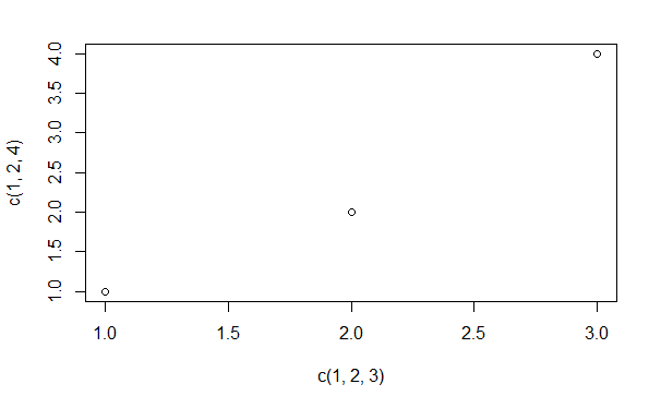
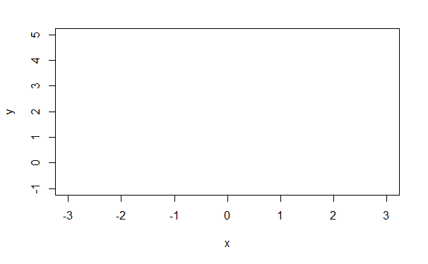
plot() 函数分阶段执行。type="n" 表示不添加任何元素
plot(
  c(-3, 3),
  c(-1, 5),
  type="n",
  xlab="x",
  ylab="y"
)
添加线条:abline() 函数
abline() 使用截距和斜率绘制直线
x <- 1:3
y <- c(1, 3, 8)
plot(x, y)
lmout <- lm(y ~ x)
abline(lmout)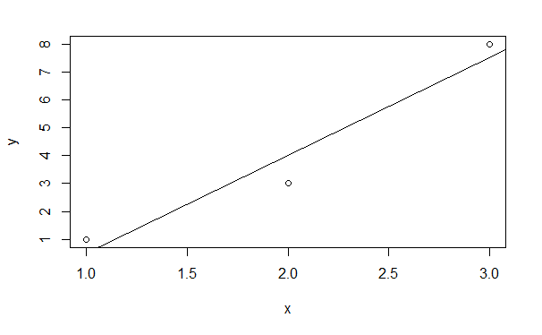
$$ y = 2 + 1 \cdot x $$
plot(
  c(-3, 3),
  c(-1, 5),
  type="n",
  xlab="x",
  ylab="y"
)
abline(c(2, 1))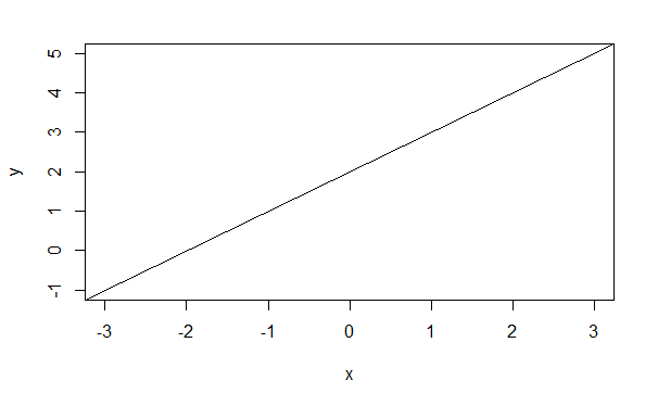
lines() 函数
plot(
  c(1, 3),
  c(2, 4),
  type="n",
  xlab="x",
  ylab="y"
)
lines(c(1.5, 2.5), c(3, 3))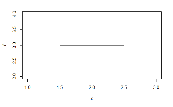
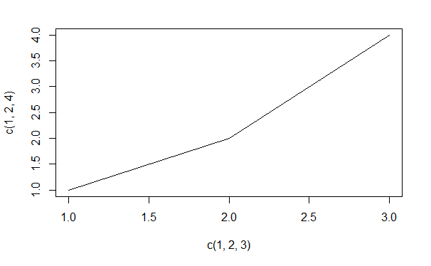
plot(
  c(1, 2, 3),
  c(1, 2, 4),
  type="l"
)
扩展案例:在一张图中绘制两条密度曲线
density() 函数计算密度曲线的估计值
scores <- read.csv("../data/student-mat.csv", header=TRUE)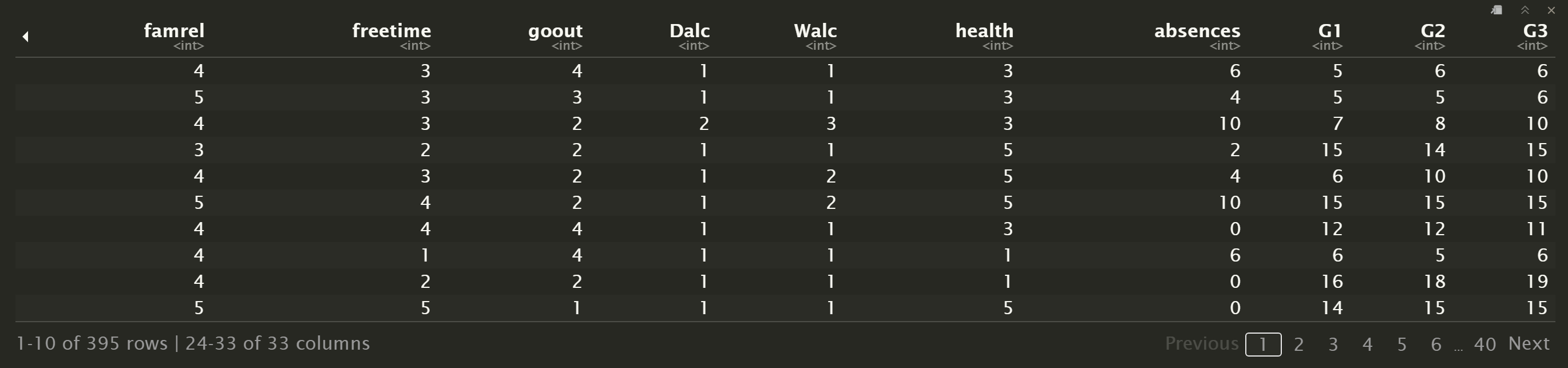
d1 <- density(scores$G1, from=0, to=20)
d2 <- density(scores$G2, from=0, to=20)
plot(d2, main="", xlab="")
lines(d1)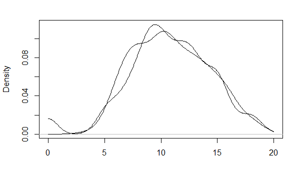
添加点:points() 函数
plot(
  c(0, 20), c(0, 20),
  type="n",
  xlab="G1",
  ylab="G3"
)
points(scores$G1, scores$G3, pch="+")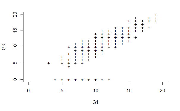
添加图例:legend() 函数
example(legend)添加文字:text() 函数
plot(d2, main="", xlab="")
lines(d1)
text(6, 0.10, "G1")
text(7, 0.03, "G2")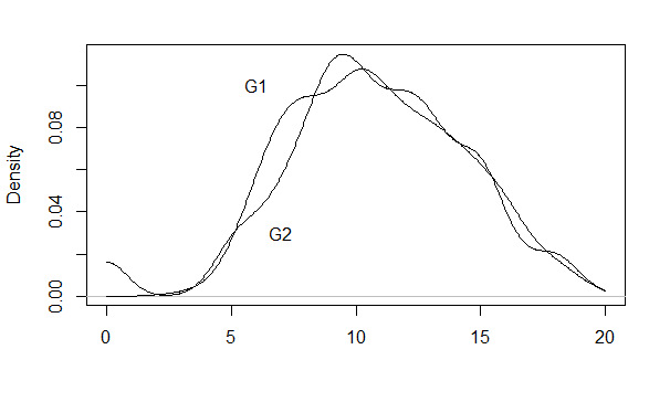
定制图形
改变字符大小:cex 选项
plot(d2, main="", xlab="")
lines(d1)
text(6, 0.10, "G1", cex=1.5)
text(7, 0.03, "G2")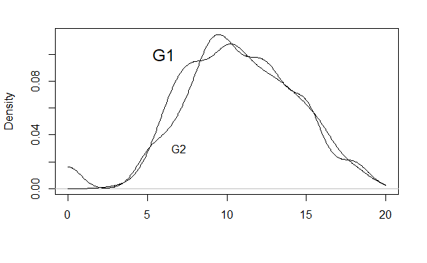
改变坐标轴的范围:xlim 和 ylim 选项
d1Call:
density.default(x = scores$G1, from = 0, to = 20)
Data: scores$G1 (395 obs.); Bandwidth 'bw' = 0.9036
x y
Min. : 0 Min. :4.650e-06
1st Qu.: 5 1st Qu.:8.764e-03
Median :10 Median :5.102e-02
Mean :10 Mean :4.989e-02
3rd Qu.:15 3rd Qu.:8.868e-02
Max. :20 Max. :1.076e-01
d2Call:
density.default(x = scores$G2, from = 0, to = 20)
Data: scores$G2 (395 obs.); Bandwidth 'bw' = 0.8126
x y
Min. : 0 Min. :0.0005023
1st Qu.: 5 1st Qu.:0.0140315
Median :10 Median :0.0405683
Mean :10 Mean :0.0490951
3rd Qu.:15 3rd Qu.:0.0865223
Max. :20 Max. :0.1146588
plot(
  c(0, 20),
  c(0, 0.12),
  type="n",
  xlab="score",
  ylab="density"
)
lines(d1)
lines(d2)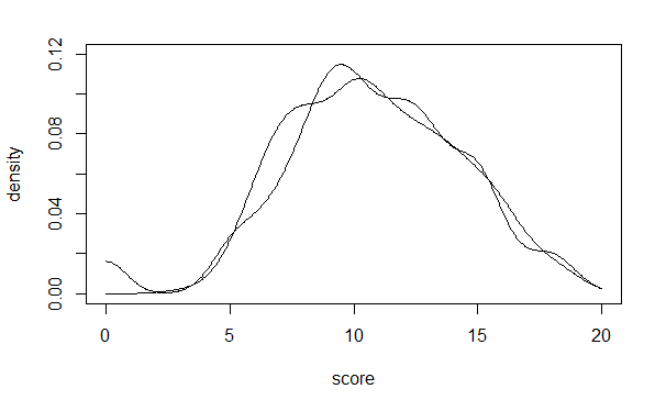
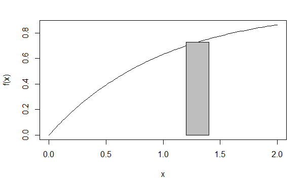
添加多边形:polygon() 函数
f <- function(x) return (1 - exp(-x))
curve(f, 0, 2)
polygon(
  c(1.2, 1.4, 1.4, 1.2),
  c(0, 0, f(1.3), f(1.3)),
  col="gray"
)
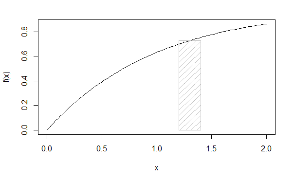
density 参数可以配置以条纹形式绘图
f <- function(x) return (1 - exp(-x))
curve(f, 0, 2)
polygon(
  c(1.2, 1.4, 1.4, 1.2),
  c(0, 0, f(1.3), f(1.3)),
  col="gray",
  density=10
)
平滑散点:lowess() 和 loess() 函数
plot(scores$G1, scores$G2)
lines(lowess(scores$G1, scores$G2))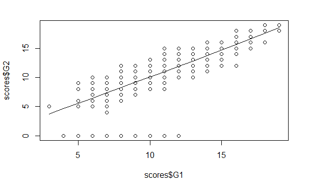
绘制具显式表达式的函数
$$ g(t) = \sqrt {t^2 + 1} $$
g <- function(t) return ((t^2 + 1)^0.5)
x <- seq(0, 5, length=10000)
y <- g(x)
plot(x, y, type="l")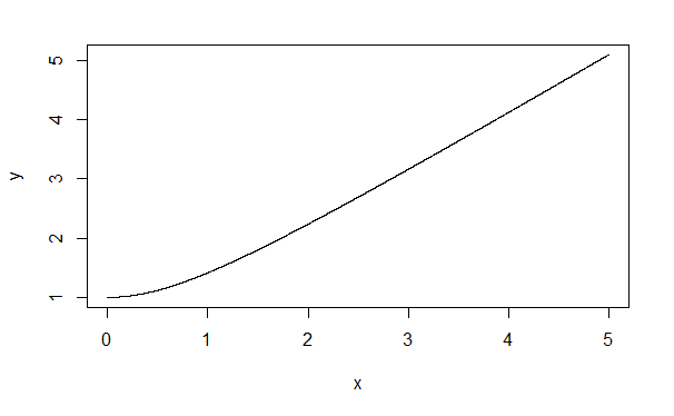
curve() 函数
curve((x^2+1)^0.5, 0, 5)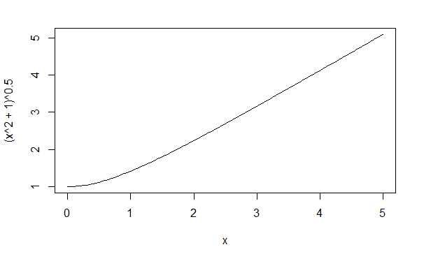
plot.function() 函数
f <- function(x) return ((x^2 + 1)^0.5)
plot(f, 0, 5)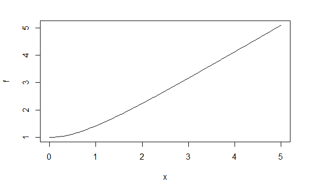
将图形保存到文件
pdf("p1.pdf")
pdf("p2.pdf")dev.list()pdf pdf
2 3
dev.set(2)pdf
2
dev.off()pdf
3
dev.set(3)pdf
3
dev.off()null device
1
创建三维图形
library(lattice)
a <- 1:10
b <- 1:15
eg <- expand.grid(x=a, y=b)
eg$z <- eg$x^2 + eg$x * eg$y
wireframe(z ~ x + y, eg)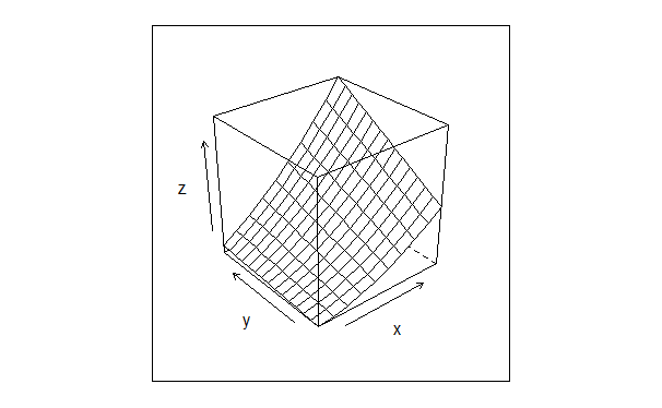
参考
学习 R 语言系列文章:
《快速入门》
《向量》
《矩阵和数组》
《列表》
《数据框》
《因子和表》
《编程结构》
《数学运算与模拟》
《面向对象编程》
《输入与输出》
《字符串操作》
本文代码请访问如下项目: