预测雷暴旋转的深度学习解释 - 数据

November 11, 2020 (最后修改: August 22, 2021)

本文翻译自 AMS 机器学习 Python 教程，并有部分修改。
Lagerquist, R., and D.J. Gagne II, 2019: “Interpretation of deep learning for predicting thunderstorm rotation: Python tutorial”.
https://github.com/djgagne/ams-ml-python-course/blob/master/module_4/ML_Short_Course_Module_4_Interpretation.ipynb

本节着重于卷积神经网络 (convolutional neural networks, CNN) 的解释，这是一种深度学习模型，用于预测来自 NCAR (National Center for Atmospheric Research) convection-allowing ensemble 的数值模拟雷暴中的未来旋转 (Schwartz et al. 2015)。

解释和理解模型在机器学习 (machine learning, ML) 的所有三个阶段都有好处：

开发阶段：可以用于调试
运行阶段：可以增加用户对模型的信任和理解
机器学习阶段：机器学习大大胜过人类的假想阶段可以用来提高人类的技能。对于国际象棋 (Johns et al. 2015) 和围棋 (Silver et al. 2016) 的游戏已经做到了这一点。

参考文献

本文引用了下面列出的一些出版物。

Breiman, L., 2001: “Random forests.” Machine Learning, 45, 5–32, https://doi.org/10.1023/A:1010933404324.

Dosovitskiy, A., and T. Brox, 2016: “Inverting visual representations with convolutional networks.” Conference on Computer Vision and Pattern Recognition, Las Vegas, Nevada, IEEE.

Hsu, W., and A. Murphy, 1986: “The attributes diagram: A geometrical framework for assessing the quality of probability forecasts.” International Journal of Forecasting, 2, 285–293, https://doi.org/10.1016/0169-2070(86)90048-8.

Johns, E., O. Aodha, and G. Brostow, 2015: “Becoming the Expert: Interactive multi-class machine teaching.” Conference on Computer Vision and Pattern Recognition, Boston, Massachusetts, IEEE.

Lakshmanan, V., C. Karstens, J. Krause, K. Elmore, A. Ryzhkov, and S. Berkseth, 2015: “Which polarimetric variables are important for weather/no-weather discrimination?” Journal of Atmospheric and Oceanic Technology, 32, 1209-1223, https://doi.org/10.1175/JTECH-D-13-00205.1.

Metz, C., 1978: “Basic principles of ROC analysis.” Seminars in Nuclear Medicine, 8, 283–298, https://doi.org/10.1016/S0001-2998(78)80014-2.

Niculescu-Mizil, A., and R. Caruana, 2005: “Predicting good probabilities with supervised learning.” International Conference on Machine Learning, Bonn, Germany, International Machine Learning Society.

Olah, C., A. Mordvintsev, and L. Schubert, 2017: “Feature visualization.” Distill, https://doi.org/10.23915/distill.00007.

Roebber, P., 2009: “Visualizing multiple measures of forecast quality.” Weather and Forecasting, 24, 601-608, https://doi.org/10.1175/2008WAF2222159.1.

Schwartz, C., G. Romine, M. Weisman, R. Sobash, K. Fossell, K. Manning, and S. Trier, 2015: “A real-time convection-allowing ensemble prediction system initialized by mesoscale ensemble Kalman filter analyses.” Weather and Forecasting, 30 (5), 1158-1181.

Selvaraju, R., M. Cogswell, A. Das, R. Vedantam, D. Parikh, and D. Batra, 2017: “Grad-CAM: Visual explanations from deep networks via gradient-based localization.” International Conference on Computer Vision, Venice, Italy, IEEE.

Silver, D., and Coauthors, 2016: “Mastering the game of Go with deep neural networks and tree search.” Nature, 529 (7587), 484–489.

Simonyan, K., A. Vedaldi, and A. Zisserman, 2014: “Deep inside convolutional networks: Visualising image classification models and saliency maps.” arXiv e-prints, 1312, https://arxiv.org/abs/1312.6034.

Wagstaff, K., and J. Lee: “Interpretable discovery in large image data sets.” arXiv e-prints, 1806, https://arxiv.org/abs/1806.08340.

Zhou, B., A. Khosla, A. Lapedriza, A. Oliva, and A. Torralba, 2016: “Learning deep features for discriminative localization.” Conference on Computer Vision and Pattern Recognition, Las Vegas, Nevada, IEEE.

安装

本文需要安装以下包：

scipy
TensorFlow
Keras
scikit-image
netCDF4
pyproj
scikit-learn
opencv-python
matplotlib
shapely
geopy
metpy
descartes

导入

导入本文将使用的所有库

import typing
import pathlib
import time
import copy
import json

import numpy as np
import pandas as pd
import xarray as xr
import matplotlib
import matplotlib.pyplot as plt
import netCDF4
from tqdm.auto import tqdm
import sklearn.metrics

import tensorflow as tf
import tensorflow.compat.v1.keras as keras
import tensorflow.compat.v1.keras.backend as K

配置 tensorflow

config_object = tf.compat.v1.ConfigProto()
config_object.gpu_options.allow_growth = True
session_object = tf.compat.v1.Session(config=config_object)

K.set_session(session_object)

注意：

已修改部分源码，放到 windroc 包中。为了更专注任务，后续仅介绍部分源码。

from windroc import utils

训练，验证和测试

模块 2 讨论了将数据集分为训练 (training)，验证 (validation) 和测试集 (testing) 的重要性。简要重申：

训练集的角色：训练模型，例如调整 CNN 中的权重
验证集的角色：选择最佳的超参数 (不由训练调整的参数)
- CNN 示例：卷积层数，每层通道数，激活函数，丢弃率等。
- 将会在本文稍后部分了解上述所有内容
测试集的角色：根据独立数据评估所选模型
- 所选模型是对验证数据表现最佳的模型

查找输入文件

注：本文数据的下载方法请查阅《AMS机器学习课程：数据分析与预处理》

查找用于训练 (2010-14) 和验证 (2015) 阶段的输入文件。本节不关心测试数据，因为我们不进行超参数实验。 CNN 的训练时间很长，超参数实验将花费更多的时间。

实现

find_many_image_files() 函数根据起止时间寻找文件路径

def find_many_image_files(
    first_date: pd.Timestamp, 
    last_date: pd.Timestamp,
    image_dir_name: str=utils.DEFAULT_IMAGE_DIR_NAME
) -> typing.List:
    netcdf_file_pattern = (
        f'{image_dir_name}/'
        f'NCARSTORM_{utils.DATE_FORMAT_REGEX}-0000_d01_model_patches.nc'
    )

    netcdf_file_names = list(pathlib.Path().glob(netcdf_file_pattern))
    netcdf_file_names.sort()
    
    # `_image_file_name_to_date()` 函数从文件名中提取日期
    file_dates = pd.Series([
        utils._image_file_name_to_date(f) 
        for f in netcdf_file_names
    ])

    good_indices = np.where(
        np.logical_and(
            file_dates >= first_date,
            file_dates <= last_date
        )
    )[0]

    return [
        netcdf_file_names[k] 
        for k in good_indices
    ]

训练集

寻找训练集文件列表

training_file_names = find_many_image_files(
    first_date=pd.to_datetime('2010-01-01'), 
    last_date=pd.to_datetime('2014-12-31'),
)
training_file_names[:5]

[WindowsPath('../data/track_data_ncar_ams_3km_nc_small/NCARSTORM_20101024-0000_d01_model_patches.nc'),
 WindowsPath('../data/track_data_ncar_ams_3km_nc_small/NCARSTORM_20101122-0000_d01_model_patches.nc'),
 WindowsPath('../data/track_data_ncar_ams_3km_nc_small/NCARSTORM_20110201-0000_d01_model_patches.nc'),
 WindowsPath('../data/track_data_ncar_ams_3km_nc_small/NCARSTORM_20110308-0000_d01_model_patches.nc'),
 WindowsPath('../data/track_data_ncar_ams_3km_nc_small/NCARSTORM_20110326-0000_d01_model_patches.nc')]

验证集

寻找验证集文件列表

validation_file_names = find_many_image_files(
    first_date=pd.to_datetime('2015-01-01'), 
    last_date=pd.to_datetime('2015-12-31'),
)
validation_file_names[:5]

[WindowsPath('../data/track_data_ncar_ams_3km_nc_small/NCARSTORM_20150331-0000_d01_model_patches.nc'),
 WindowsPath('../data/track_data_ncar_ams_3km_nc_small/NCARSTORM_20150416-0000_d01_model_patches.nc'),
 WindowsPath('../data/track_data_ncar_ams_3km_nc_small/NCARSTORM_20150422-0000_d01_model_patches.nc'),
 WindowsPath('../data/track_data_ncar_ams_3km_nc_small/NCARSTORM_20150505-0000_d01_model_patches.nc'),
 WindowsPath('../data/track_data_ncar_ams_3km_nc_small/NCARSTORM_20150510-0000_d01_model_patches.nc')]

读取验证集数据

读取验证集数据并探索其中一个文件的内容。

我们不会一次读取所有的数据，因为训练集要大得多。根据运行环境的硬件配置，训练集可能无法一次全部放入内存中。

E：文件中样本 (风暴对象) 个数
M：每个以风暴为中心的网格的行数
N：每个以风暴为中心的网格的列数
C：通道数 (预报变量)

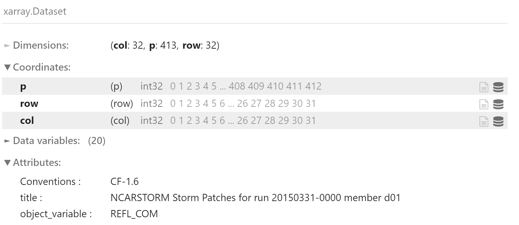
使用 xarray 加载文件

ds = xr.open_dataset(validation_file_names[0])
ds

ds.U10_curr.shape

(413, 32, 32)

使用 netCDF4 加载文件

read_image_file() 函数从 NetCDF 文件中读取以风暴为中心的图像

返回结果为字典类型

storm_ids：风暴ID，长度为 E
storm_steps：风暴步骤数，长度为 E
predictor_names：预报变量名称，长度为 C
predictor_matrix：预报变量数组，维度为 (E, M, N, C)
target_name：目标变量名称
target_matrix：目标值，维度为 (E, M, N)

def read_image_file(
    netcdf_file_name: str
) -> typing.Dict:
    dataset_object = netCDF4.Dataset(netcdf_file_name)

    storm_ids = np.array(
        dataset_object.variables[utils.NETCDF_TRACK_ID_NAME][:], 
        dtype=int
    )
    storm_steps = np.array(
        dataset_object.variables[utils.NETCDF_TRACK_STEP_NAME][:], 
        dtype=int
    )

    predictor_matrix = None

    for this_predictor_name in utils.NETCDF_PREDICTOR_NAMES:
        # 维度 (p, row, col)
        this_predictor_matrix = np.array(
            dataset_object.variables[this_predictor_name][:], 
            dtype=float
        )
        
        # 在最内维度上再增加一个维度
        # 新数据 (p, row, col, predictors)
        this_predictor_matrix = np.expand_dims(
            this_predictor_matrix, 
            axis=-1
        )

        if predictor_matrix is None:
            predictor_matrix = this_predictor_matrix + 0.
        else:
            predictor_matrix = np.concatenate(
                (predictor_matrix, this_predictor_matrix), 
                axis=-1
            )

    target_matrix = np.array(
        dataset_object.variables[utils.NETCDF_TARGET_NAME][:], 
        dtype=float
    )

    return {
        utils.STORM_IDS_KEY: storm_ids,
        utils.STORM_STEPS_KEY: storm_steps,
        utils.PREDICTOR_NAMES_KEY: utils.PREDICTOR_NAMES,
        utils.PREDICTOR_MATRIX_KEY: predictor_matrix,
        utils.TARGET_NAME_KEY: utils.TARGET_NAME,
        utils.TARGET_MATRIX_KEY: target_matrix
    }

read_many_image_files() 函数多个 NetCDF 文件中读取以风暴为中心的图像

def read_many_image_files(
    netcdf_file_names: typing.List
) -> typing.Dict:
    image_dict = None
    keys_to_concat = [
        utils.STORM_IDS_KEY, 
        utils.STORM_STEPS_KEY, 
        utils.PREDICTOR_MATRIX_KEY, 
        utils.TARGET_MATRIX_KEY
    ]

    for this_file_name in tqdm(netcdf_file_names):
        this_image_dict = read_image_file(this_file_name)

        if image_dict is None:
            image_dict = copy.deepcopy(this_image_dict)
            continue

        for this_key in keys_to_concat:
            image_dict[this_key] = np.concatenate(
                (
                    image_dict[this_key], 
                    this_image_dict[this_key]
                ), 
                axis=0
            )

    return image_dict

读取图像数据，保存到 validation_image_dict 中

validation_image_dict = read_many_image_files(validation_file_names)

validation_image_dict 中的变量

for this_key in validation_image_dict.keys():
    print(this_key)

storm_ids
storm_steps
predictor_names
predictor_matrix
target_name
target_matrix

风暴 ID 个数，即样本个数

validation_image_dict["storm_ids"].shape[0]

预测变量名

predictor_names = validation_image_dict[utils.PREDICTOR_NAMES_KEY]
for this_name in predictor_names:
    print(this_name)

reflectivity_dbz
temperature_kelvins
u_wind_m_s01
v_wind_m_s01

输入数据维度

validation_image_dict[utils.PREDICTOR_MATRIX_KEY].shape

(25392, 32, 32, 4)

目标变量名

validation_image_dict[utils.TARGET_NAME_KEY]

'max_future_vorticity_s01'

查看第一个风暴对象

第一个预测变量

predictor_names[0]

'reflectivity_dbz'

数值

validation_image_dict[utils.PREDICTOR_MATRIX_KEY][0, :5, :5, 0]

array([[20.71773911, 23.83432198, 25.17814636, 26.48272514, 24.63681602],
       [21.99064636, 24.18389511, 26.43440056, 28.80635834, 28.36290169],
       [25.46614838, 27.86122131, 29.8734417 , 31.37428093, 30.02640724],
       [27.25055885, 30.0418911 , 31.66870308, 32.69125366, 30.8074894 ],
       [26.84561729, 30.45740128, 32.21142578, 32.33716965, 30.79758072]])

目标变量

validation_image_dict[utils.TARGET_NAME_KEY]

'max_future_vorticity_s01'

validation_image_dict[utils.TARGET_MATRIX_KEY][0, :5, :5]

array([[0.00084322, 0.00080153, 0.00081101, 0.00089913, 0.00105435],
       [0.0008761 , 0.00085617, 0.00087151, 0.00093471, 0.00107364],
       [0.00081878, 0.00081321, 0.00075086, 0.00082498, 0.00105294],
       [0.00057726, 0.00057209, 0.00051179, 0.00068943, 0.000877  ],
       [0.00054895, 0.00064536, 0.00076832, 0.00098494, 0.00098583]])

绘图

绘图函数

plot_many_predictors_with_barbs() 函数绘制多个带风向杆的图形

M：行数
N：列数
C：预报变量数

predictor_matrix：形为 (M, N, C) 的数组

def plot_many_predictors_with_barbs(
    predictor_matrix: np.ndarray, 
    predictor_names: typing.List, 
    min_colour_temp_kelvins: float,
    max_colour_temp_kelvins: float,
) -> typing.Tuple[matplotlib.figure.Figure, typing.List]:
    # 提取风场，将风场添加到所有图形中
    u_wind_matrix_m_s01 = predictor_matrix[
        ..., predictor_names.index(utils.U_WIND_NAME)
    ]
    
    v_wind_matrix_m_s01 = predictor_matrix[
        ..., predictor_names.index(utils.V_WIND_NAME)
    ]
    
    # 除风场之外的变量
    non_wind_predictor_names = [
        p for p in predictor_names 
        if p not in [utils.U_WIND_NAME, utils.V_WIND_NAME]
    ]
    
    # 构造画板
    # `_init_figure_panels()` 函数初始化绘图面板
    figure_object, axes_objects_2d_list = utils._init_figure_panels(
        num_columns=len(non_wind_predictor_names), 
        num_rows=1
    )

    for m in range(len(non_wind_predictor_names)):
        this_predictor_index = predictor_names.index(
            non_wind_predictor_names[m]
        )

        if non_wind_predictor_names[m] == utils.REFLECTIVITY_NAME:
            this_colour_norm_object = utils.REFL_COLOUR_NORM_OBJECT
            this_min_colour_value = None
            this_max_colour_value = None
        else:
            this_colour_norm_object = None
            this_min_colour_value = min_colour_temp_kelvins + 0.
            this_max_colour_value = max_colour_temp_kelvins + 0.

        this_colour_bar_object = plot_predictor_2d(
            predictor_matrix=predictor_matrix[..., this_predictor_index],
            colour_map_object=utils.PREDICTOR_TO_COLOUR_MAP_DICT[
                non_wind_predictor_names[m]],
            colour_norm_object=this_colour_norm_object,
            min_colour_value=this_min_colour_value,
            max_colour_value=this_max_colour_value,
            axes_object=axes_objects_2d_list[0][m]
        )

        plot_wind_2d(
            u_wind_matrix_m_s01=u_wind_matrix_m_s01,
            v_wind_matrix_m_s01=v_wind_matrix_m_s01,
            axes_object=axes_objects_2d_list[0][m]
        )

        this_colour_bar_object.set_label(non_wind_predictor_names[m])

    return figure_object, axes_objects_2d_list

plot_predictor_2d() 函数绘制预测变量二维图形

def plot_predictor_2d(
    predictor_matrix: np.ndarray,
    colour_map_object: matplotlib.pyplot.cm,
    colour_norm_object=None,
    min_colour_value: float=None, 
    max_colour_value: float=None, 
    axes_object=None
) -> matplotlib.pyplot.colorbar:
    if axes_object is None:
        _, axes_object = plt.subplots(
            1, 1, 
            figsize=(
                utils.FIGURE_WIDTH_INCHES, 
                utils.FIGURE_HEIGHT_INCHES
            )
        )

    if colour_norm_object is not None:
        min_colour_value = colour_norm_object.boundaries[0]
        max_colour_value = colour_norm_object.boundaries[-1]

    axes_object.pcolormesh(
        predictor_matrix, 
        cmap=colour_map_object, 
        norm=colour_norm_object,
        vmin=min_colour_value,
        vmax=max_colour_value, 
        shading='flat',
        edgecolors='None'
    )

    axes_object.set_xticks([])
    axes_object.set_yticks([])
    
    # `_add_colour_bar()` 函数添加色表
    return utils._add_colour_bar(
        axes_object=axes_object, 
        colour_map_object=colour_map_object,
        values_to_colour=predictor_matrix, 
        min_colour_value=min_colour_value,
        max_colour_value=max_colour_value
    )

plot_wind_2d() 函数绘制风场图形

def plot_wind_2d(
    u_wind_matrix_m_s01: np.ndarray, 
    v_wind_matrix_m_s01: np.ndarray, 
    axes_object=None
):
    if axes_object is None:
        _, axes_object = plt.subplots(
            1, 1, 
            figsize=(
                utils.FIGURE_WIDTH_INCHES, 
                utils.FIGURE_HEIGHT_INCHES
            )
        )

    num_grid_rows = u_wind_matrix_m_s01.shape[0]
    num_grid_columns = u_wind_matrix_m_s01.shape[1]

    x_coords_unique = np.linspace(
        0, 
        num_grid_columns, 
        num=num_grid_columns + 1, 
        dtype=float
    )
    x_coords_unique = x_coords_unique[:-1]
    x_coords_unique = x_coords_unique + np.diff(x_coords_unique[:2]) / 2

    y_coords_unique = np.linspace(
        0, 
        num_grid_rows, 
        num=num_grid_rows + 1, 
        dtype=float
    )
    y_coords_unique = y_coords_unique[:-1]
    y_coords_unique = y_coords_unique + np.diff(y_coords_unique[:2]) / 2

    x_coord_matrix, y_coord_matrix = np.meshgrid(
        x_coords_unique,
        y_coords_unique
    )

    speed_matrix_m_s01 = np.sqrt(
        u_wind_matrix_m_s01 ** 2 + v_wind_matrix_m_s01 ** 2
    )

    axes_object.barbs(
        x_coord_matrix, 
        y_coord_matrix,
        u_wind_matrix_m_s01 * utils.METRES_PER_SECOND_TO_KT,
        v_wind_matrix_m_s01 * utils.METRES_PER_SECOND_TO_KT,
        speed_matrix_m_s01 * utils.METRES_PER_SECOND_TO_KT, 
        color='k', 
        length=6,
        sizes={'emptybarb': 0.1}, 
        fill_empty=True, 
        rounding=False
    )

    axes_object.set_xlim(0, num_grid_columns)
    axes_object.set_ylim(0, num_grid_rows)

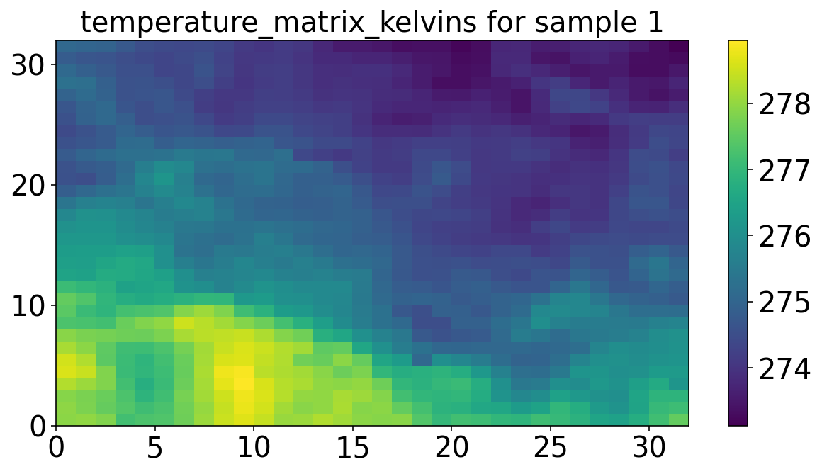
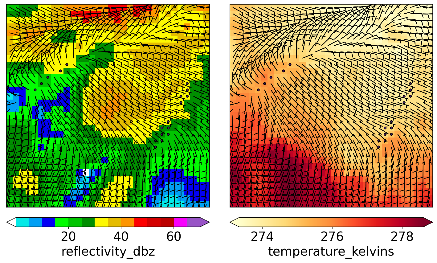
示例 1

绘制验证阶段的某个随机样本

第一个样本的数据，32 x 32 网格，4 个预测变量

predictor_matrix = validation_image_dict[utils.PREDICTOR_MATRIX_KEY][0, ...]
predictor_matrix.shape

(32, 32, 4)

预测变量名

predictor_names = validation_image_dict[utils.PREDICTOR_NAMES_KEY]
predictor_names

['reflectivity_dbz', 'temperature_kelvins', 'u_wind_m_s01', 'v_wind_m_s01']

提取温度数据，变量名 temperature_matrix_kelvins

temperature_matrix_kelvins = predictor_matrix[
    ..., predictor_names.index(utils.TEMPERATURE_NAME)
]

plt.figure(figsize=(10, 5))
plt.pcolormesh(temperature_matrix_kelvins)
plt.colorbar()
plt.title("temperature_matrix_kelvins for sample 1")
plt.show()

绘制图形

plot_many_predictors_with_barbs(
    predictor_matrix=predictor_matrix,
    predictor_names=predictor_names,
    min_colour_temp_kelvins=np.percentile(temperature_matrix_kelvins, 1),
    max_colour_temp_kelvins=np.percentile(temperature_matrix_kelvins, 99)
)
plt.show()

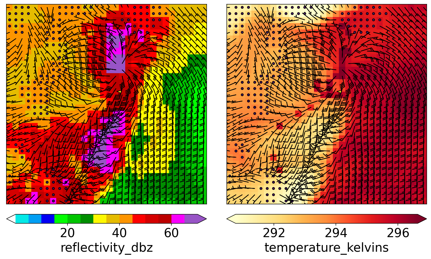
示例 2

绘制验证集的最强示例（未来涡度最大）。

target_matrix_s01 = validation_image_dict[utils.TARGET_MATRIX_KEY]
target_matrix_s01.shape

(25392, 32, 32)

查找最大值，获取样本索引

example_index = np.unravel_index(
    np.argmax(target_matrix_s01), 
    target_matrix_s01.shape
)[0]
example_index

获取样本数据

predictor_matrix = validation_image_dict[utils.PREDICTOR_MATRIX_KEY][
    example_index, ...]
predictor_matrix.shape

(32, 32, 4)

提取温度数据

predictor_names = validation_image_dict[utils.PREDICTOR_NAMES_KEY]
temperature_matrix_kelvins = predictor_matrix[
    ..., predictor_names.index(utils.TEMPERATURE_NAME)
]

绘制图像

plot_many_predictors_with_barbs(
    predictor_matrix=predictor_matrix,
    predictor_names=predictor_names,
    min_colour_temp_kelvins=np.percentile(temperature_matrix_kelvins, 1),
    max_colour_temp_kelvins=np.percentile(temperature_matrix_kelvins, 99)
)

plt.show()

归一化

在模块 2 中讨论了归一化预测变量的重要性。简要重申一下：

当有多个不同尺度的预测变量时，应将其归一化。这样可以确保模型不会忽略较小比例的变量。

例如，如果模型以开尔文为单位的温度和单位为 kg kg^-1 的湿度进行训练，则模型可能会学会强调温度 (大约180-330 K)，并忽略湿度 (大约0-0.02 kg kg^-1)。

实现

仅基于训练数据，计算每个预测变量的归一化参数 (均值和标准差)。

使用这些平均值和标准偏差对训练和验证集进行归一化。

对训练数据进行反归一化，并确保反归一化的值=原始值 (合理性检查)。

get_image_normalization_params() 计算归一化参数

def get_image_normalization_params(
    netcdf_file_names: typing.List
) -> typing.Dict:
    predictor_names = None
    norm_dict_by_predictor = None

    for this_file_name in tqdm(netcdf_file_names):
        this_image_dict = read_image_file(this_file_name)

        if predictor_names is None:
            predictor_names = this_image_dict[utils.PREDICTOR_NAMES_KEY]
            norm_dict_by_predictor = [{}] * len(predictor_names)

        for m in range(len(predictor_names)):
            norm_dict_by_predictor[m] = _update_normalization_params(
                intermediate_normalization_dict=norm_dict_by_predictor[m],
                new_values=this_image_dict[utils.PREDICTOR_MATRIX_KEY][..., m]
            )

    normalization_dict = {}

    for m in range(len(predictor_names)):
        this_mean = norm_dict_by_predictor[m][utils.MEAN_VALUE_KEY]
        this_stdev = _get_standard_deviation(norm_dict_by_predictor[m])

        normalization_dict[predictor_names[m]] = np.array(
            [this_mean, this_stdev]
        )

        print(
            f'Mean and standard deviation for "{predictor_names[m]}" '
            f'= {this_mean:.4f}, {this_stdev:.4f}'
        )

    return normalization_dict

_update_normalization_params() 函数为一个预测变量更新归一化参数。

intermediate_normalization_dict 包含以下字段：

num_values：当前估计值所基于数据量
mean_value：当前估计的均值
mean_of_squares：当前估计的均方值

该函数用于动态更新归一化参数，可以不用将所有数据全部载入到内存中

def _update_normalization_params(
    intermediate_normalization_dict: typing.Dict, 
    new_values: np.ndarray
) -> typing.Dict:
    if utils.MEAN_VALUE_KEY not in intermediate_normalization_dict:
        intermediate_normalization_dict = {
            utils.NUM_VALUES_KEY: 0,
            utils.MEAN_VALUE_KEY: 0.,
            utils.MEAN_OF_SQUARES_KEY: 0.
        }

    these_means = np.array([
        intermediate_normalization_dict[utils.MEAN_VALUE_KEY], 
        np.mean(new_values)
    ])
    these_weights = np.array([
        intermediate_normalization_dict[utils.NUM_VALUES_KEY], 
        new_values.size
    ])

    intermediate_normalization_dict[utils.MEAN_VALUE_KEY] = np.average(
        these_means, weights=these_weights)

    these_means = np.array([
        intermediate_normalization_dict[utils.MEAN_OF_SQUARES_KEY],
        np.mean(new_values ** 2)
    ])

    intermediate_normalization_dict[utils.MEAN_OF_SQUARES_KEY] = np.average(
        these_means, weights=these_weights)

    intermediate_normalization_dict[utils.NUM_VALUES_KEY] += new_values.size
    return intermediate_normalization_dict

_get_standard_deviation() 函数计算标准差

def _get_standard_deviation(
    intermediate_normalization_dict: typing.Dict
) -> float:
    num_values = float(intermediate_normalization_dict[utils.NUM_VALUES_KEY])
    multiplier = num_values / (num_values - 1)

    return np.sqrt(multiplier * (
        intermediate_normalization_dict[utils.MEAN_OF_SQUARES_KEY] -
        intermediate_normalization_dict[utils.MEAN_VALUE_KEY] ** 2
    ))

计算归一化参数

normalization_dict = get_image_normalization_params(
    training_file_names
)
normalization_dict

Mean and standard deviation for "reflectivity_dbz" = 22.6855, 15.7617
Mean and standard deviation for "temperature_kelvins" = 290.3430, 7.6134
Mean and standard deviation for "u_wind_m_s01" = -0.2901, 4.6689
Mean and standard deviation for "v_wind_m_s01" = 0.8431, 5.0262
{'reflectivity_dbz': array([22.68552537, 15.76168208]),
 'temperature_kelvins': array([290.34299022,   7.61342361]),
 'u_wind_m_s01': array([-0.29011941,  4.66887569]),
 'v_wind_m_s01': array([0.84309994, 5.0262159 ])}

验证

normalize_images() 函数用于对数据进行归一化

predictor_matrix 参数维度 (examples, rows, columns, channels)

def normalize_images(
    predictor_matrix: np.ndarray, 
    predictor_names: typing.List, 
    normalization_dict: typing.Optional[typing.Dict]=None
) -> typing.Tuple[np.ndarray, typing.Dict]:
    num_predictors = len(predictor_names)

    if normalization_dict is None:
        normalization_dict = {}

        for m in range(num_predictors):
            this_mean = np.mean(predictor_matrix[..., m])
            this_stdev = np.std(predictor_matrix[..., m], ddof=1)

            normalization_dict[predictor_names[m]] = np.array(
                [this_mean, this_stdev]
            )

    for m in range(num_predictors):
        this_mean = normalization_dict[predictor_names[m]][0]
        this_stdev = normalization_dict[predictor_names[m]][1]

        predictor_matrix[..., m] = (
            (predictor_matrix[..., m] - this_mean) / float(this_stdev)
        )

    return predictor_matrix, normalization_dict

denormalize_images() 函数实现反归一化

def denormalize_images(
    predictor_matrix: np.ndarray, 
    predictor_names: typing.List, 
    normalization_dict: typing.Dict
) -> np.ndarray:
    num_predictors = len(predictor_names)

    for m in range(num_predictors):
        this_mean = normalization_dict[predictor_names[m]][0]
        this_stdev = normalization_dict[predictor_names[m]][1]

        predictor_matrix[..., m] = (
            this_mean + this_stdev * predictor_matrix[..., m]
        )

    return predictor_matrix

选取第一个样本验证归一化过程是否正确

first_training_image_dict = read_image_file(training_file_names[0])

第一个预报变量

first_training_image_dict[utils.PREDICTOR_NAMES_KEY][0]

'reflectivity_dbz'

预报变量的原始值，截取 5x5 范围

these_predictor_values = (
    first_training_image_dict[utils.PREDICTOR_MATRIX_KEY][0, :5, :5, 0]
)
these_predictor_values

array([[ 0.        ,  6.9651885 ,  6.99899673,  3.64286256,  0.        ],
       [ 1.818367  ,  4.22854471,  0.28074482,  0.        ,  0.        ],
       [ 7.24424314,  4.46407127,  0.        ,  0.        ,  0.        ],
       [16.65088844, 18.46622086, 17.29220772, 13.19463634,  2.80103612],
       [19.96715736, 22.98410988, 23.0850563 , 19.88584709, 11.70358849]])

归一化后的值

first_training_image_dict[utils.PREDICTOR_MATRIX_KEY], _ = (
    normalize_images(
        predictor_matrix=first_training_image_dict[
            utils.PREDICTOR_MATRIX_KEY
        ],
        predictor_names=predictor_names,
        normalization_dict=normalization_dict
    )
)

these_predictor_values = (
    first_training_image_dict[utils.PREDICTOR_MATRIX_KEY][0, :5, :5, 0]
)
these_predictor_values

array([[-1.43928327, -0.99737685, -0.99523189, -1.20816184, -1.43928327],
       [-1.32391697, -1.17100323, -1.42147142, -1.43928327, -1.43928327],
       [-0.97967223, -1.15606025, -1.43928327, -1.43928327, -1.43928327],
       [-0.38286757, -0.2676938 , -0.34217907, -0.6021495 , -1.26157152],
       [-0.17246687,  0.0189437 ,  0.02534824, -0.1776256 , -0.69674904]])

反归一化后恢复的值

first_training_image_dict[utils.PREDICTOR_MATRIX_KEY] = (
    denormalize_images(
        predictor_matrix=first_training_image_dict[
            utils.PREDICTOR_MATRIX_KEY
        ],
        predictor_names=predictor_names,
        normalization_dict=normalization_dict
    )
)

these_predictor_values = (
    first_training_image_dict[utils.PREDICTOR_MATRIX_KEY][0, :5, :5, 0]
)
these_predictor_values

array([[ 0.        ,  6.9651885 ,  6.99899673,  3.64286256,  0.        ],
       [ 1.818367  ,  4.22854471,  0.28074482,  0.        ,  0.        ],
       [ 7.24424314,  4.46407127,  0.        ,  0.        ,  0.        ],
       [16.65088844, 18.46622086, 17.29220772, 13.19463634,  2.80103612],
       [19.96715736, 22.98410988, 23.0850563 , 19.88584709, 11.70358849]])

二元分类

回归 (regression) 和分类 (classification) 之间的区别已在模块 2 中讨论。本文重申：

本模块的其余部分着重于二元分类 (binary classification)，而不是回归。 “回归”是对实数的预测 (例如，我们预测最大未来涡度)。 “分类”是对类别的预测 (例如，低，中或高的最大未来涡度)。

二元分类中有两个类别。因此，预测采取回答是或否问题的形式。除了将其二值化外，我们将使用相同的目标变量 (最大未来涡度，max future vorticity)。问题将是预测最大未来涡度是否超过阈值。

计算阈值

本节将目标变量“二值化”：将每个值转换为 0 或 1，是或否。

阈值是所有训练示例中最大未来涡度的第 90% 分位数。

对训练集和验证集使用相同的阈值进行二值化。

get_binarization_threshold() 函数计算阈值

def get_binarization_threshold(
    netcdf_file_names: typing.List, 
    percentile_level: float
) -> float:
    max_target_values = np.array([])

    for this_file_name in tqdm(netcdf_file_names):
        this_image_dict = read_image_file(this_file_name)

        this_target_matrix = this_image_dict[utils.TARGET_MATRIX_KEY]
        this_num_examples = this_target_matrix.shape[0]
        
        these_max_target_values = np.full(
            this_num_examples, 
            np.nan
        )
        
        # 每个样本的最大值
        for i in range(this_num_examples):
            these_max_target_values[i] = np.max(
                this_target_matrix[i, ...]
            )

        max_target_values = np.concatenate((
            max_target_values, 
            these_max_target_values
        ))

    binarization_threshold = np.percentile(
        max_target_values, 
        percentile_level
    )

    return binarization_threshold

计算阈值

binarization_threshold = get_binarization_threshold(
    netcdf_file_names=training_file_names, 
    percentile_level=90.
)
binarization_threshold

0.005431033764034511

计算分类

第一个文件中前 10 个样本的目标变量

first_training_image_dict = read_image_file(training_file_names[0])
these_max_target_values = np.array([
    np.max(
        first_training_image_dict[utils.TARGET_MATRIX_KEY][i, ...]
    )
    for i in range(10)
])
these_max_target_values

array([0.0021904 , 0.00241288, 0.00241288, 0.00245462, 0.00258843,
       0.00216414, 0.001725  , 0.00137892, 0.00147138, 0.00117736])

binarize_target_images() 函数计算分类

target_matrix 维度 (examples, rows, columns)

def binarize_target_images(
    target_matrix: np.ndarray, 
    binarization_threshold: float,
) -> np.ndarray:
    num_examples = target_matrix.shape[0]
    target_values = np.full(
        num_examples, 
        -1, 
        dtype=int
    )

    for i in range(num_examples):
        target_values[i] = (
            np.max(target_matrix[i, ...]) 
            >= 
            binarization_threshold
        )

    return target_values

计算分类

target_values = binarize_target_images(
    target_matrix=first_training_image_dict[utils.TARGET_MATRIX_KEY],
    binarization_threshold=binarization_threshold
)
target_values[:10]