Dask应用：使用 Dask 并行抽取站点数据

November 02, 2020 (最后修改: September 25, 2021)

meteorology/data, programming/python

本文介绍如何使用 Dask 从多个文件中提取站点垂直廓线和剖面图数据。

简介

最近在构建面向冬奥会服务的 GRAPES MESO 1KM 产品后处理的 ecFlow 系统 (grapes_meso_1km_post)。

模式生成数据的信息如下：

纬度 latitude：44.5 - 34.5
经度 longitude：108 - 124
分辨率：0.01 度，1km
格点数 ni * nj：1601 * 1601
时效 step：0 - 24 小时，逐小时间隔
层次 pl：15 个等压面层，从 1000 hPa 到 100 hPa

其中一种产品是站点预报产品，包括：

站点的垂直廓线数据
经过站点的沿经线和纬线的垂直剖面图数据

该数据由原始分辨率 GRIB 2 数据文件抽取生成，所有时效和所有变量都包含在同一个 NetCDF 文件中。一共有 9 种变量，每种变量 3 类数据，每类数据 25 个时效，每个时效包含 15 层。

当前任务脚本使用 NCL 抽取数据并输出 NetCDF 文件。经集成测试，每个站点的任务运行耗时均在 70 分钟左右。对于计划逐小时运行的模式系统来说，这可能不是一个理想的运行时间。

因为 ecFlow 系统需要保证前一天最后一个任务的完成时间要早于下一天第一个任务的启动时间，才能持续滚动循环。
当然，任何系统都有实现的方式。只要将系统拆分为多个 ecFlow 系统，就可以规避时间重叠的问题。只不过这通常不是最佳实践。

本文首先介绍 NCL 脚本的实现方法，再介绍笔者使用 Dask 库进行并行抽取的尝试。

使用 NCL 提取

GRAPES 模式输出的 GRIB 2 文件分时效保存。 NCL 脚本首先使用 addfiles 命令批量打开 GRIB 2 文件。

inputf = addfiles(input_filename,"r")

为所有要素场申请空间。下面代码是位势高度的示例代码，其中 hgt_0 和 hgt_9 保存剖面图数据，hgt 保存廓线图数据。所有数据前两个维度都是时效和层次。

hgt_0=new((/dimsizes(time),dimsizes(level),interp_0/),"float")
hgt_9=new((/dimsizes(time),dimsizes(level),interp_9/),"float")
hgt=new((/dimsizes(time),dimsizes(level)/),"float")

从每个时效文件中依次读取要素场，填充到数据数组中。

do i=0,dimsizes(time)-1
    hgt_0(i,:,:)=inputf[i]->HGT_P0_L100_GLL0(:,180:860:-1,797)
    hgt_9(i,:,:)=inputf[i]->HGT_P0_L100_GLL0(:,405,520:1220)
    hgt(i,:)=inputf[i]->HGT_P0_L100_GLL0(:,405,797)
    ; ...skip...
end do

最后当所有数据数组填充完毕后，将数据写入到 NetCDF 文件中。

实际测试时，上述每次 do 循环大约耗时 3 分钟，一共 25 次，所以总耗时将近 75 分钟。

笔者不熟悉 NCL，不清楚 NCL 读取 GRIB 2 文件的性能。

为了更好比较运行时间，下面首先用 nwpc-oper/nwpc-data 库重新实现上述的串行加载过程。

使用 nwpc-data 库

以下代码均在 CMA-PI 上运行。

首先载入需要的库

import pathlib

import numpy as np
import xarray as xr
from tqdm.auto import tqdm

from nwpc_data.grib.eccodes import load_field_from_file

数据

获取数据文件列表

data_path = pathlib.Path("/g11/wangdp/project/work/data/playground/station/ncl/data/grib2-orig")
files = list(data_path.glob("rmf.hgra.*.grb2"))
files = sorted(files)

站点信息

站点和剖面图数据的范围均使用维度坐标的序号表示。

station_lat_index = 405
station_lon_index = 797

lat_index_range = (180, 861)
lon_index_range = (520, 1221)

要素

names = [
    "gh",
    "q",
    "r",
    "t",
    "u",
    "v",
    "wz",
    "snmr",
    "clwmr",
]

抽取函数

使用 isel() 方法根据维度坐标序号抽取数据

get_station() 函数获取站点廓线图数据

def get_station(field):
    field_station = field.isel(
        latitude=station_lat_index, 
        longitude=station_lon_index
    )
    return field_station

get_lat_section() 函数获取站点纬向剖面图数据

def get_lat_section(field):
    field_lat_section = field.isel(
        latitude=slice(*lat_index_range),
        longitude=station_lon_index,
    )[:,::-1]
    return field_lat_section

get_lon_section() 函数获取站点经向剖面图数据

def get_lon_section(field):
    field_lon_section = field.isel(
        latitude=station_lat_index,
        longitude=slice(*lon_index_range),
    )
    return field_lon_section

combine_fields() 函数将多个单时效的要素场合并为同一个对象，增加 step 维度

def combine_fields(fields):
    return xr.concat(fields, dim="step")

串行执行

下面代码串行获取所需数据，保存到 data_list 字典对象中

data_list = dict()
for field_name in tqdm(names):
    stations = []
    lat_sections = []
    lon_sections = []
    for file_path in tqdm(files):
        field = load_field_from_file(
            file_path,
            parameter=field_name,
            level_type="pl"
        )
        field_station = get_station(field)
        field_lat_section = get_lat_section(field)
        field_lon_section = get_lon_section(field)
        stations.append(field_station)
        lat_sections.append(field_lat_section)
        lon_sections.append(field_lon_section)
        
    data_list[f"{field_name}"] = combine_fields(stations)
    data_list[f"{field_name}_0"] = combine_fields(lat_sections)
    data_list[f"{field_name}_9"] = combine_fields(lon_sections)

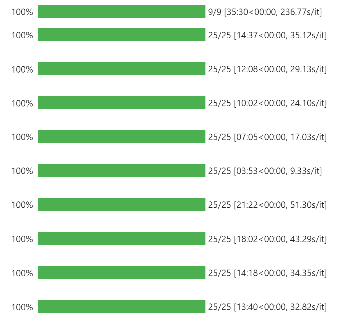
从下图可以看到载入全部要素场需要 35 分钟

合并数据

查看已加载的数据

for item in data_list.keys():
    print(item)

gh
gh_0
gh_9
q
q_0
q_9
r
r_0
r_9
t
t_0
t_9
u
u_0
u_9
v
v_0
v_9
wz
wz_0
wz_9
snmr
snmr_0
snmr_9
clwmr
clwmr_0
clwmr_9

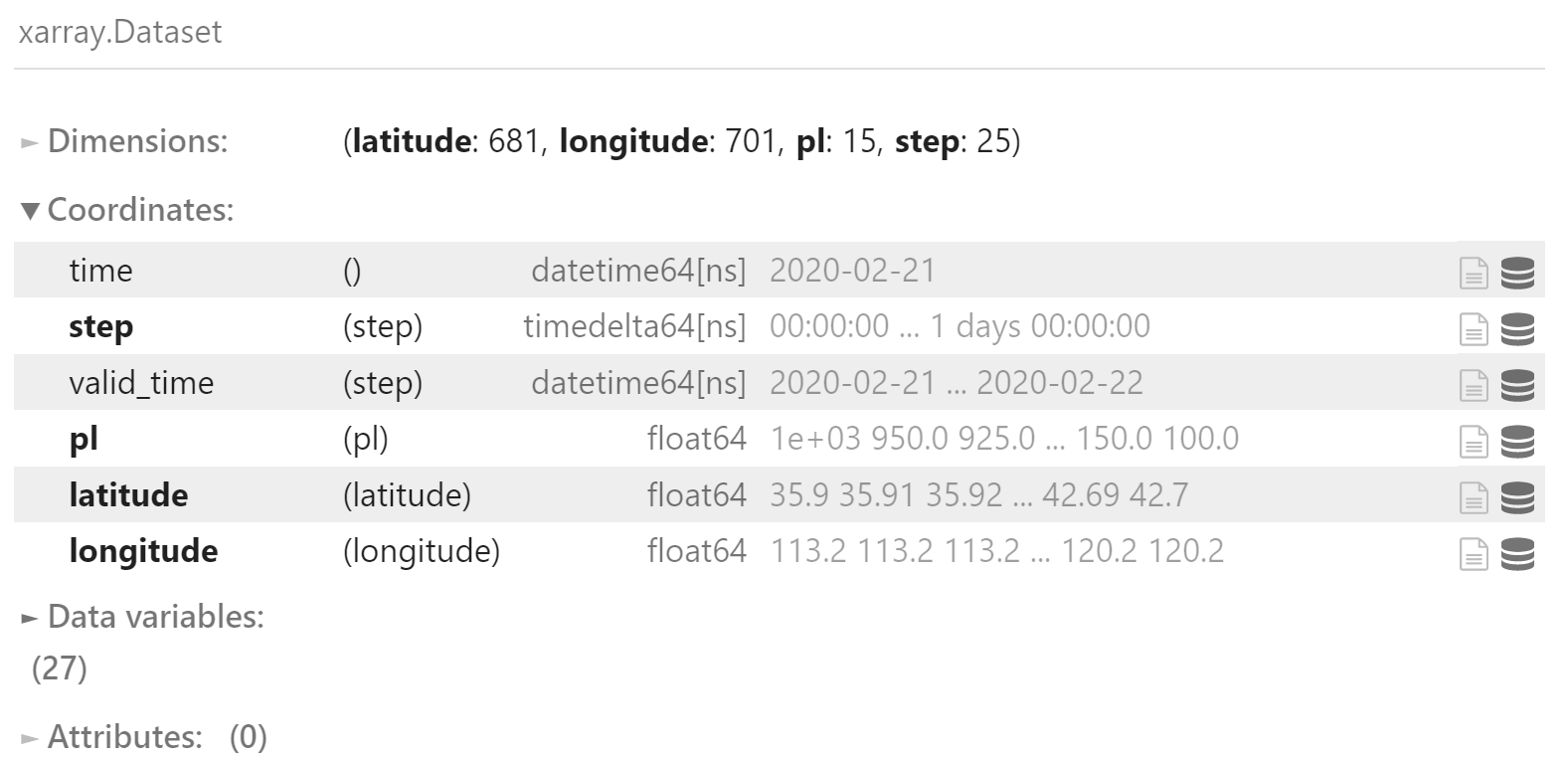
将全部数据合并为单个 xr.Dataset 对象

ds = xr.Dataset(data_list)
ds

写入到 NetCDF 文件中

可以将 xarray.Dataset 对象直接写入到 NetCDF 文件中

ds.to_netcdf("ds.nc")

使用 Dask

上节的串行执行部分代码中有两重 for 循环，是最核心的耗时操作。可以使用 Dask 库对 for 循环进行改造，实现简单的并行算法。

准备

载入需要使用的库

import dask
from dask.distributed import Client, progress

在登录节点启动 Dask 客户端，下面的代码启动 8 个进程，共 32 个线程。

n_workers = 8
client = Client(
    n_workers=n_workers,
)
client

并行改造

对 for 循环中的耗时函数，改用 dask.delayed() 函数延迟执行

从 GRIB 2 中读取要素场：load_field_from_file
从要素场中抽取数据：get_station，get_lat_section 和 get_lon_section
合并多时效要素场：combine_fields

data_list = dict()
for field_name in names:
    stations = []
    lat_sections = []
    lon_sections = []
    for file_path in files:
        field = dask.delayed(load_field_from_file)(
            file_path,
            parameter=field_name,
            level_type="pl"
        )
        field_station = dask.delayed(get_station)(field)
        field_lat_section = dask.delayed(get_lat_section)(field)
        field_lon_section = dask.delayed(get_lon_section)(field)
        stations.append(field_station)
        lat_sections.append(field_lat_section)
        lon_sections.append(field_lon_section)
        
    data_list[f"{field_name}"] = dask.delayed(combine_fields)(stations)
    data_list[f"{field_name}_0"] = dask.delayed(combine_fields)(lat_sections)
    data_list[f"{field_name}_9"] = dask.delayed(combine_fields)(lon_sections)

另外，dask.delayed 需要一个单一的计算目标用于完成整个计算。所以将 data_list 封装到函数中

def get_data_list(data_list):
    return data_list

最终的计算目标来自 get_data_list() 函数

t = dask.delayed(get_data_list)(data_list)

执行

执行整个流程，使用 progress() 显示计算进度

result = t.persist()
progress(result)

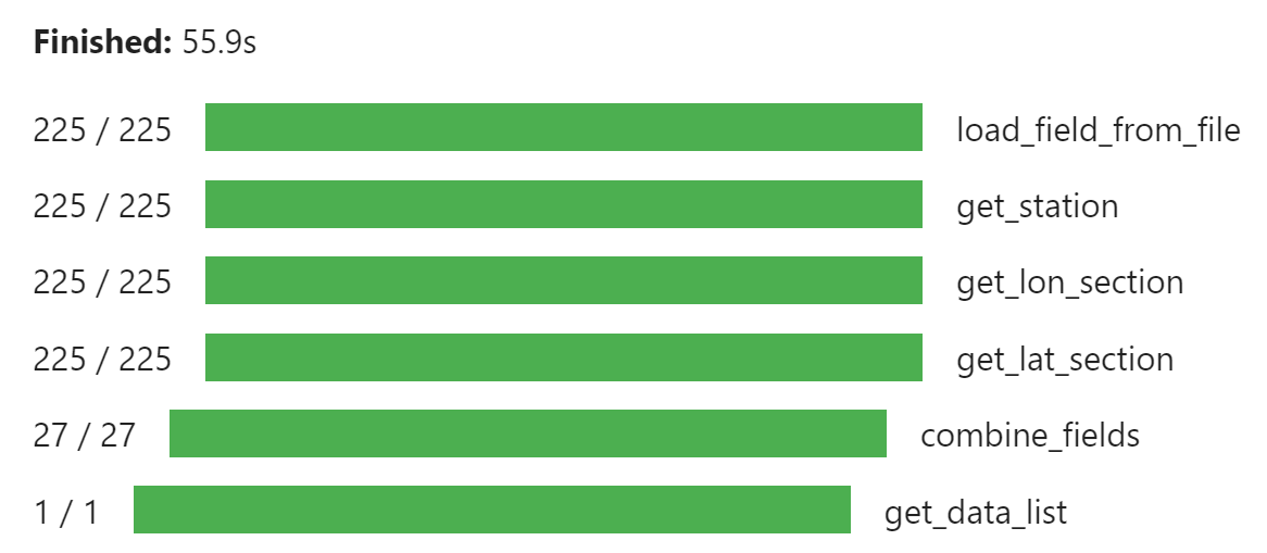
由上图可见，使用 Dask 并行抽取可以大幅度提高数据处理速度。

获取结果

compute() 函数可以获取最终的计算结果

r = result.compute()

r 实际上就是串行版本中的 data_list，可以构建 xr.Dataset 对象，并输出到 NetCDF 文件中。

讨论

使用 Dask 改写 for 循环是一种非常简便的并行算法实现方式。

当然，本文代码还有进一步改进的空间：

生成的 NetCDF 文件与 NCL 生成的文件内容不完全一致，需要进一步调整维度坐标等内容。

仅在登录节点上运行无法充分利用 HPC 的并行计算能力，需要尝试在并行计算节点中运行 Dask 脚本。

参考

nwpc-data 项目：

《nwpc-data 库简介》

https://github.com/nwpc-oper/nwpc-data

nwpc-data 使用 eccodes-python 加载多层数据，详情请参考以下文章

《GRIB笔记：使用cfgrib加载垂直剖面图数据》

《GRIB笔记：使用eccodes-python加载垂直剖面图数据》

Dask：

下面的文章也使用 Dask 对 for 循环进行改造：

《计算等压面要素场检验指标 - 并发》