计算地面要素场基本检验指标
本文以 2 米温度为例,说明如何根据站点观测计算地面要素场的检验指标。
重要提示:本文使用的数据均来自其他工具。
准备
载入需要使用到的库
import numpy as np
import xarray as xr
import pandas as pd
import geopandas as gpd

import matplotlib.pyplot as plt

import pathlib

from nwpc_data.grib.eccodes import (
    load_field_from_file
)
数据
计算检验指标最关键的步骤就是准备数据。
本文仅使用下面子区域中的数据
domain = [20, 55, 70, 145]
观测数据
使用现有的观测数据,每个时次一个文件。
原始观测数据来自从 CIMISS 检索的全球地面逐小时数据 (SURF_GLB_MUL_HOR)。
下面是一个时次的样例文件
2016070112    08652
61902     -7.97    345.60   1019.20     26.60     17.90    150.00      8.20 999999.00 999999.00 999999.00 999999.00
10147     53.63      9.99   1011.90     18.70     15.98    210.00      6.30      0.10      0.10 999999.00   1010.10
10162     53.64     11.39   1012.30     22.10     14.95    210.00      6.60      0.00      0.00 999999.00   1005.40
10184     54.10     13.41   1013.20     24.20     12.68    230.00      4.50      0.00      0.00 999999.00   1012.40
第一行是时次和条目数。
第二行开始是每个站点的观测数据。包括以下 12 个字段(括号中是 CIMISS 的要素代码):
- 站号 (Station_Id_d)
- 纬度 (Lat)
- 经度 (Lon)
- 海平面气压 (PRS_Sea)
- 温度 (TEM)
- 露点温度 (DPT)
- 风向 (WIN_D)
- 风速 (WIN_S)
- 1小时降水 (PRE_1h)
- 6小时降水 (PRE_6h)
- 24小时降水 (PRE_24h)
- 气压 (PRS)
其中 999999.00 是缺测值
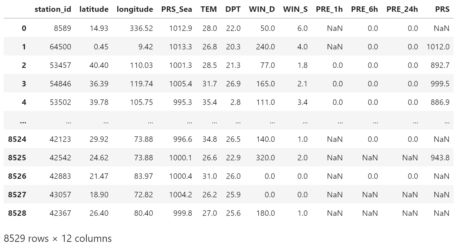
load_obs 函数用于加载观测数据。
使用 read_csv 读取等宽文本中的数据,并将缺失值 999999.0 替换为 np.nan
def load_obs(file_path: str or pathlib.Path) -> pd.DataFrame:
    columns_name = [
        "station_id",
        "latitude",
        "longitude",
        "PRS_Sea",
        "TEM",
        "DPT",
        "WIN_D",
        "WIN_S",
        "PRE_1h",
        "PRE_6h",
        "PRE_24h",
        "PRS",
    ]
    obs_file = open(file_path, "r")
    obs_file.readline()
    df = pd.read_csv(
        obs_file,
        sep="\s+",
        names=columns_name,
    )
    obs_file.close()
    df[df==999999.0] = np.nan
    return df
加载数据
obs_file_path = "/obs-base-path/201607/gts2016072912.txt"

df = load_obs(obs_file_path)
df
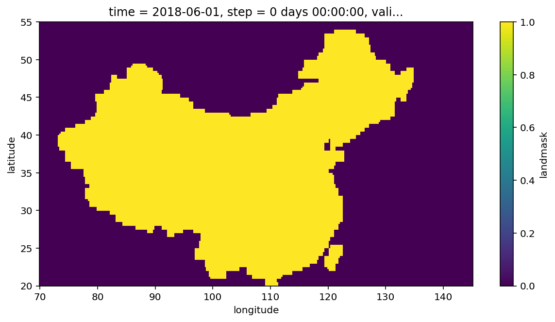
陆地掩码数据
本文仅统计部分区域的站点,所以进一步使用了掩码数据从 domain 矩形区域中提取数据。
掩码数据是一个 GRIB 2 消息,分辨率与模式数据保持一致。
mask_file_path = "/project/landmask.grib"
!grib_ls {mask_file_path}
/project/landmask.grib
edition      centre       typeOfLevel  level        dataDate     stepRange    shortName    packingType  gridType
1            0            surface      0            20180601     0            unknown      grid_simple  regular_ll
1 of 1 messages in /project/landmask.grib

1 of 1 total messages in 1 files
使用 nwpc-data 库加载掩码场
mask_field = load_field_from_file(
    mask_file_path,
    parameter=None,
)
mask_field.attrs["long_name"] = "landmask"
绘制 domain 区域的掩码场
mask_field.sel(
    latitude=slice(20, 55),
    longitude=slice(70, 145)
).plot(
    figsize=(10, 5)
)
plt.show()
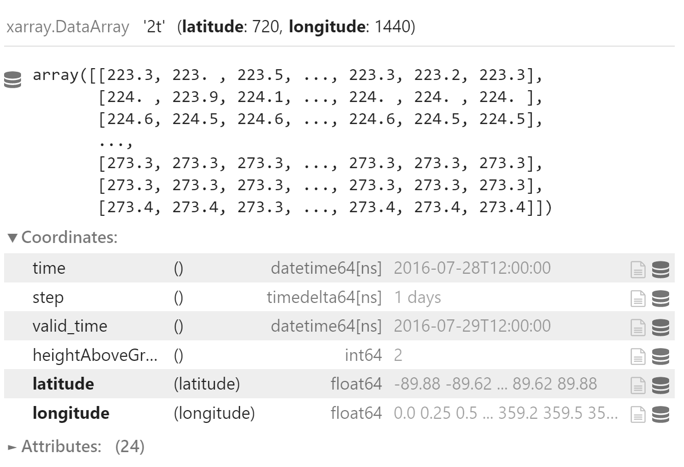
预报数据
以某试验 024 时效 2 米温度要素场为例
已将 2 米温度提取到单独的文件中
t2m_file_path = "/project/CTL/t2m024.grapes.2016072812"
!grib_ls {t2m_file_path}
/project/CTL/t2m024.grapes.2016072812
edition      centre       typeOfLevel  level        dataDate     stepRange    shortName    packingType  gridType
1            kwbc         heightAboveGround  2            20160728     24           2t           grid_simple  regular_ll
1 of 1 messages in /project/CTL/t2m024.grapes.2016072812

1 of 1 total messages in 1 files
加载温度场
t2m_field = load_field_from_file(
    t2m_file_path,
    parameter="2t",
)
t2m_field
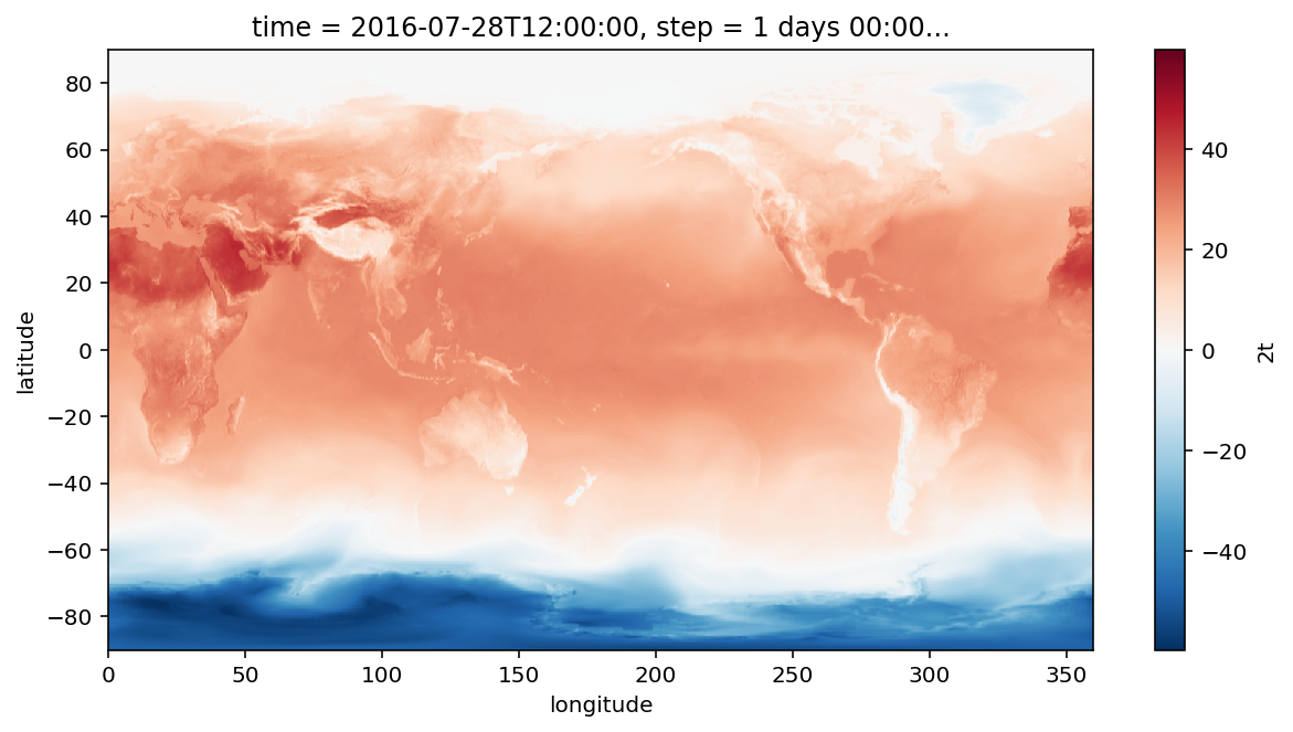
绘制温度数据
(t2m_field - 273.15).plot(figsize=(10, 5))
plt.show()
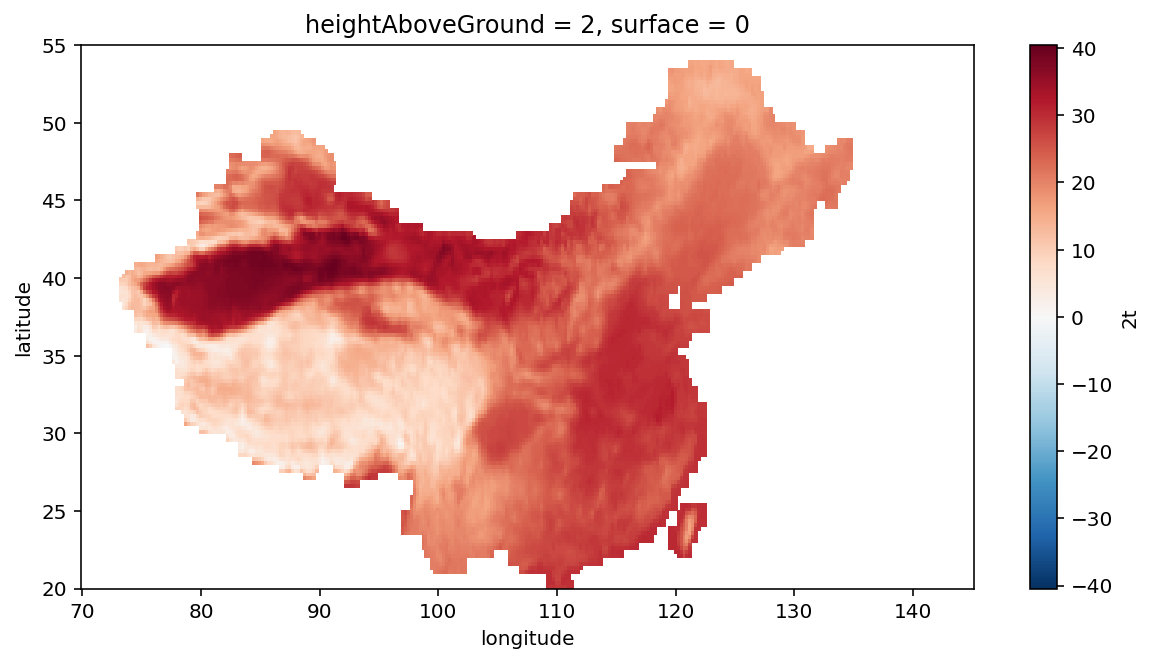
在 domain 区域范围内按掩码文件选择的数据,并绘图
(t2m_field - 273.15).where(
    mask_field == 1
).sel(
    longitude=slice(70, 145),
    latitude=slice(20, 55),
).plot(figsize=(10, 5))
plt.show()
按掩码文件选择数据,其余格点被设为 np.nan
注意:这里没有按区域裁剪,因为区域内观测站点对应的最近邻点可能在区域外(可能在本例中没有这样的点)
t2m_area = (t2m_field - 273.15).where(
    mask_field == 1
)
处理数据
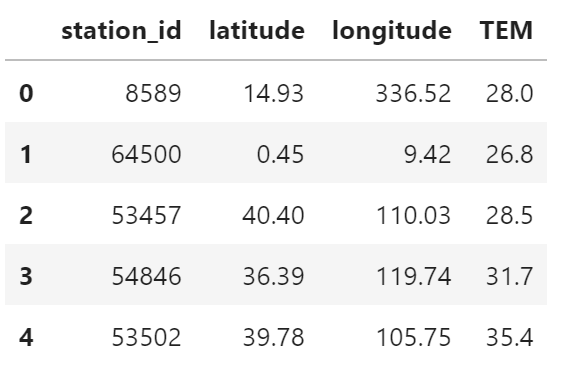
只保留温度数据,并忽略缺失值
temperature = df[df["TEM"].notna()][
    ["station_id", "latitude", "longitude", "TEM"]
]
temperature.head()
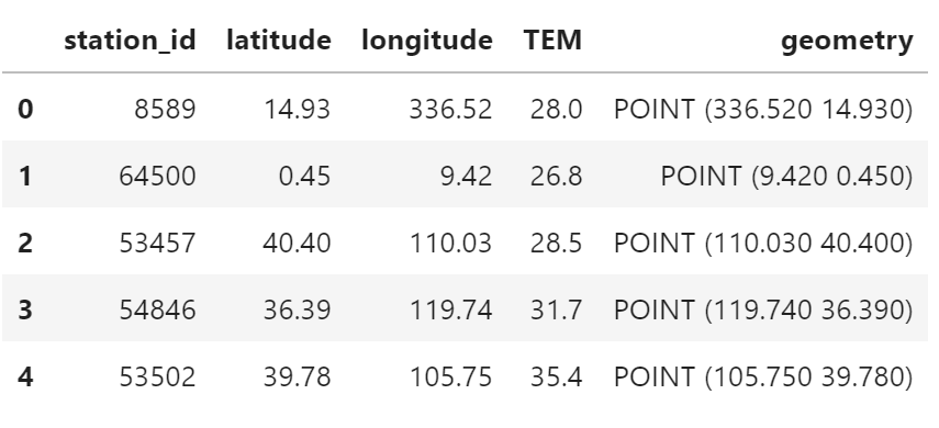
使用 latitude 和 longitude 字段构建 geopandas.GeoDataFrame 对象
geo_temperature = gpd.GeoDataFrame(
    temperature,
    geometry=gpd.points_from_xy(
        temperature.longitude,
        temperature.latitude
    )
)
geo_temperature.head()
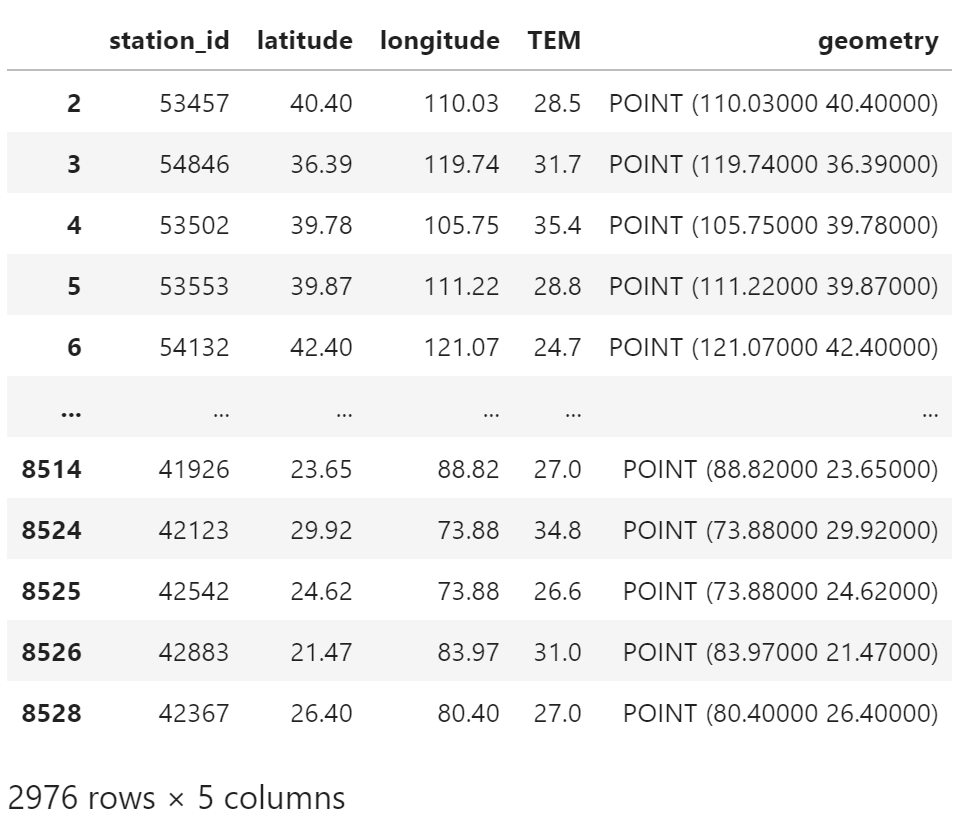
选择 domain 区域范围内的观测值
from shapely.geometry import Point, Polygon

polygen = Polygon([
    (70, 20),
    (70, 55),
    (145, 55),
    (145, 20),
])

area_temperature = geo_temperature[geo_temperature.intersects(polygen)].copy()
area_temperature
为每个站点添加预报场中最近邻点的值。
注意:因为预报场使用了掩码处理,所以值可能为 np.nan
def get_forecast(line):
    value = t2m_area.sel(
        longitude=line["longitude"],
        latitude=line["latitude"],
        method="nearest"
    ).item()
    return value

area_temperature["forecast"] = area_temperature.apply(
    get_forecast,
    axis="columns"
)
去掉 nan 值
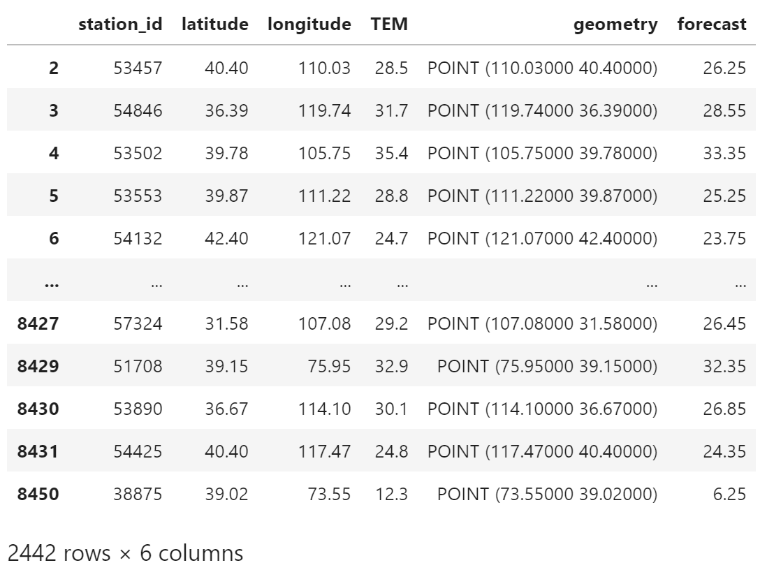
df_area = area_temperature.dropna()
df_area
计算指标
已有的计算结果
TIME    RMSE      BIAS     ABIAS
 24     4.00     -3.05     3.35
RMSE
np.sqrt(
    np.power(
        df_area["forecast"] - df_area["TEM"],
        2
    ).mean()
)
3.9974544008833273
ME
(df_area["forecast"] - df_area["TEM"]).mean()
-3.046969696969662
MAE
(df_area["forecast"] - df_area["TEM"]).abs().mean()
3.354013104013076
计算结果与已有结果保持一致。
参考
https://github.com/nwpc-oper/nwpc-data
