预测雷暴旋转的基础机器学习：分类 - 决策树超参数试验

August 30, 2020 (最后修改: August 22, 2021)

本文翻译自 AMS 机器学习 Python 教程，并有部分修改。
Lagerquist, R., and D.J. Gagne II, 2019: “Basic machine learning for predicting thunderstorm rotation: Python tutorial”. https://github.com/djgagne/ams-ml-python-course/blob/master/module_2/ML_Short_Course_Module_2_Basic.ipynb.

本文接上一篇文章《预测雷暴旋转的基础机器学习：分类 - 决策树》，介绍如何通过超参数试验确定决策树的最小样本量。

简介

两个超参数（以及其他）控制决策树的深度：

每个分支节点的最小样本量 (N_{b}^{min})
每个叶节点的最小样本量 (N_{l}^{min})

如果将这些值设置为 1，则树可能会变得很深，从而增加其过拟合的能力。

您可以用另一种方式思考：如果每个叶节点上只有一个示例，则所有预测都将仅基于一个示例，并且可能无法很好地推广到新数据。

相反，如果将 N_{b}^{min} 和 N_{l}^{min} 设置得过高，则树将变得不够深，从而导致树欠拟合。

例如，假设有 1000 个训练样本并将 N_{l}^{min} 设置为 1000。这将只允许一个分支节点（根节点）。根节点的两个子节点都具有 <1000 个示例。因此，预测将仅基于一个问题。

回顾超参数试验的四个步骤

选择要尝试的值

我们尝试

\begin{equation*} N_b^{\textrm{min}} \in \lbrace 2, 5, 10, 20, 30, 40, 50, 100, 200, 500 \rbrace \end{equation*}

和

\begin{equation*} N_l^{\textrm{min}} \in \lbrace 1, 5, 10, 20, 30, 40, 50, 100, 200, 500 \rbrace \end{equation*}

但是我们不尝试 N_{l}^{min} >= N_{b}^{min} 的组合，因为这样没有意义（N 个样本节点的子节点不可能有 >= N 个样本）

使用每种组合训练模型
在验证集上评估每个模型
选择对验证数据表现最佳的模型。
在这里，我们将“最佳”定义为 Brier 技能评分最高。

训练

下一个单元格执行超参数实验的步骤 1 和 2（定义要尝试的值并训练模型）。

定义要尝试的值

min_per_split_values = np.array(
    [2, 5, 10, 20, 30, 40, 50, 100, 200, 500], 
    dtype=int
)

min_per_leaf_values = np.array(
    [1, 5, 10, 20, 30, 40, 50, 100, 200, 500], 
    dtype=int
)

准备空白的评分数组

num_min_per_split_values = len(min_per_split_values)
num_min_per_leaf_values = len(min_per_leaf_values)

validation_auc_matrix = np.full(
    (num_min_per_split_values, num_min_per_leaf_values), 
    np.nan
)

validation_max_csi_matrix = validation_auc_matrix + 0.
validation_bs_matrix = validation_auc_matrix + 0.
validation_bss_matrix = validation_auc_matrix + 0.

计算平均观测频率

training_event_frequency = np.mean(
    training_target_table[BINARIZED_TARGET_NAME].values
)
training_event_frequency

0.10034434450161697

训练样本，并计算在验证集上的评分

from tqdm.notebook import trange, tqdm

with tqdm(range(num_min_per_split_values)) as split_t:
    for i in split_t:
        split_value = min_per_split_values[i]
        split_t.set_description(f"split ({split_value})")
        with tqdm(range(num_min_per_leaf_values), leave=False) as leaf_t:
            for j in leaf_t:
                leaf_value = min_per_leaf_values[j]
                leaf_t.set_description(f"leaf ({leaf_value})")
                if leaf_value >= split_value:
                    continue
                
                current_model = setup_classification_tree(
                    min_examples_at_split=split_value,
                    min_examples_at_leaf=leaf_value
                )
        
                _ = train_classification_tree(
                    model=current_model,
                    training_predictor_table=training_predictor_table,
                    training_target_table=training_target_table,
                )
        
                these_validation_predictions = current_model.predict_proba(
                    validation_predictor_table.values
                )[:, 1]
        
                current_evaluation_dict = eval_binary_classifn(
                    observed_labels=validation_target_table[BINARIZED_TARGET_NAME].values,
                    forecast_probabilities=these_validation_predictions,
                    training_event_frequency=training_event_frequency,
                    create_plots=False, 
                    verbose=False,
                )
        
                validation_auc_matrix[i, j] = current_evaluation_dict[AUC_KEY]
                validation_max_csi_matrix[i, j] = current_evaluation_dict[MAX_CSI_KEY]
                validation_bs_matrix[i, j] = current_evaluation_dict[BRIER_SCORE_KEY]
                validation_bss_matrix[i, j] = current_evaluation_dict[BRIER_SKILL_SCORE_KEY]

验证

下一个单元格执行超参数实验的步骤 3（在验证数据上评估每个模型）。

plot_scores_2d 函数绘制二维网格评分图，已在《预测雷暴旋转的基础机器学习 - 超参数试验》中介绍。

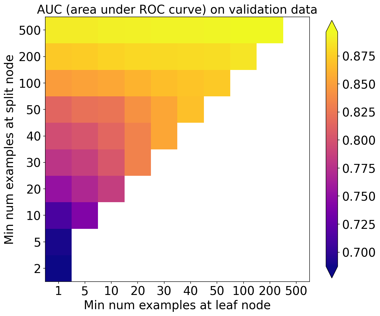
AUC

plot_scores_2d(
    score_matrix=validation_auc_matrix,
    min_colour_value=np.nanpercentile(validation_auc_matrix, 1.),
    max_colour_value=np.nanpercentile(validation_auc_matrix, 99.),
    x_tick_labels=min_per_leaf_values,
    y_tick_labels=min_per_split_values,
)

pyplot.xlabel('Min num examples at leaf node')
pyplot.ylabel('Min num examples at split node')
pyplot.title('AUC (area under ROC curve) on validation data')
pyplot.show()

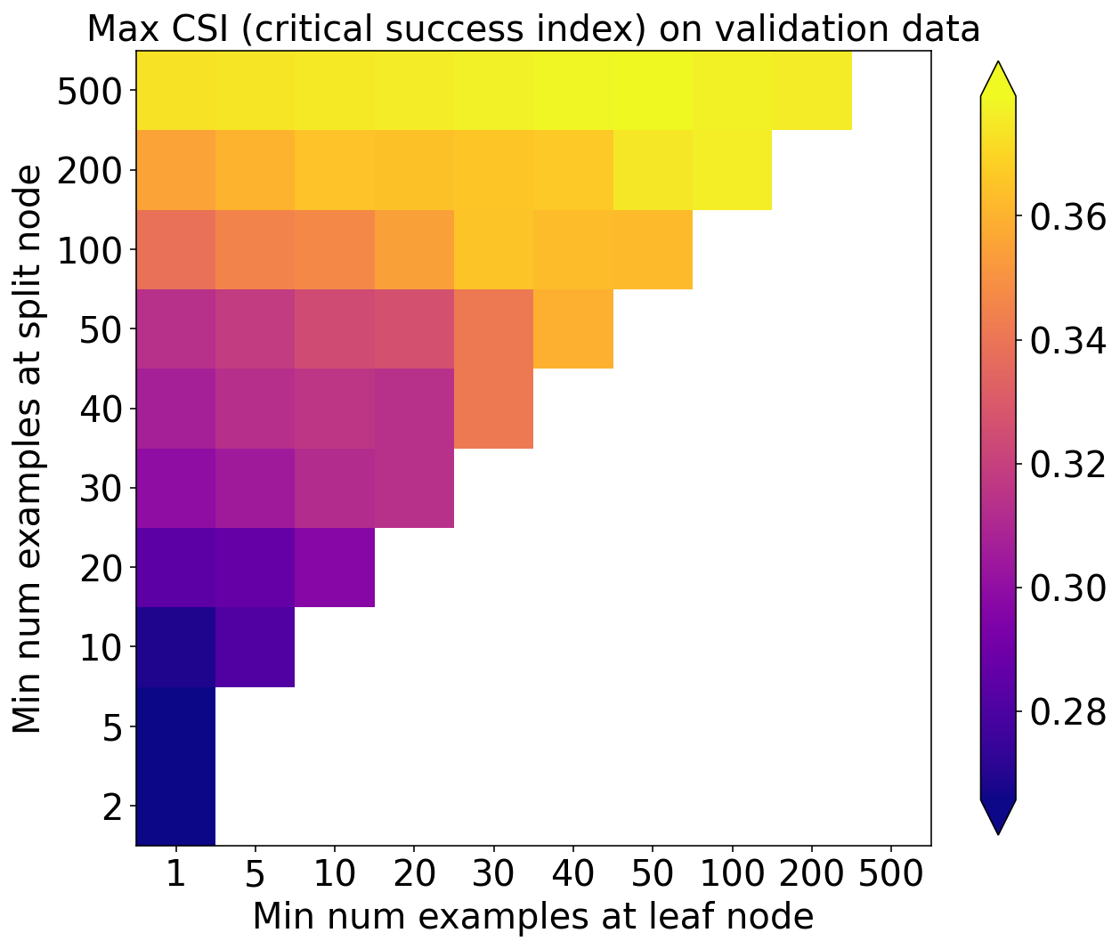
Max CSI

plot_scores_2d(
    score_matrix=validation_max_csi_matrix,
    min_colour_value=np.nanpercentile(validation_max_csi_matrix, 1.),
    max_colour_value=np.nanpercentile(validation_max_csi_matrix, 99.),
    x_tick_labels=min_per_leaf_values,
    y_tick_labels=min_per_split_values
)

pyplot.xlabel('Min num examples at leaf node')
pyplot.ylabel('Min num examples at split node')
pyplot.title('Max CSI (critical success index) on validation data')
pyplot.show()

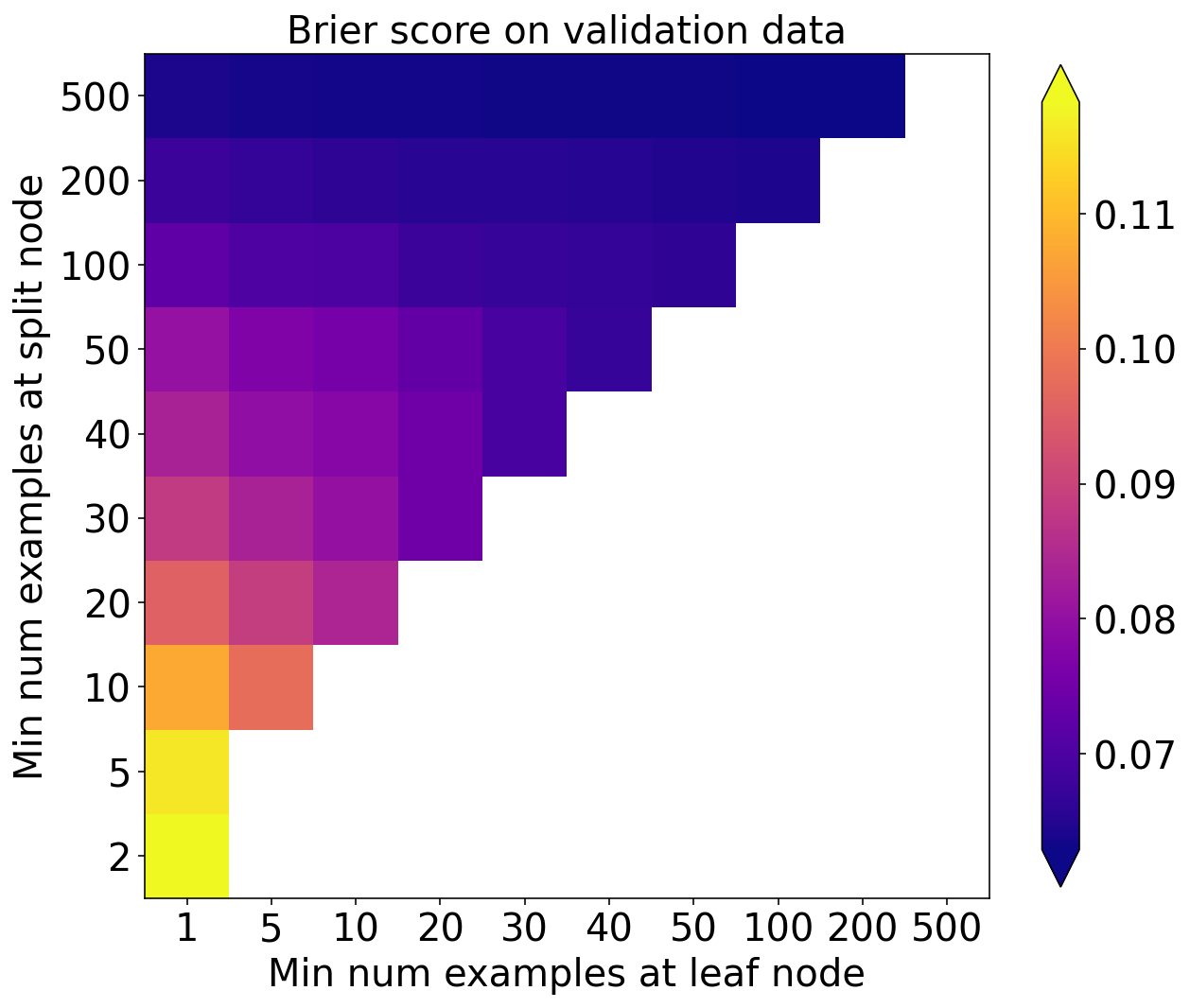
Brier score

plot_scores_2d(
    score_matrix=validation_bs_matrix,
    min_colour_value=np.nanpercentile(validation_bs_matrix, 1.),
    max_colour_value=np.nanpercentile(validation_bs_matrix, 99.),
    x_tick_labels=min_per_leaf_values,
    y_tick_labels=min_per_split_values
)

pyplot.xlabel('Min num examples at leaf node')
pyplot.ylabel('Min num examples at split node')
pyplot.title('Brier score on validation data')
pyplot.show()

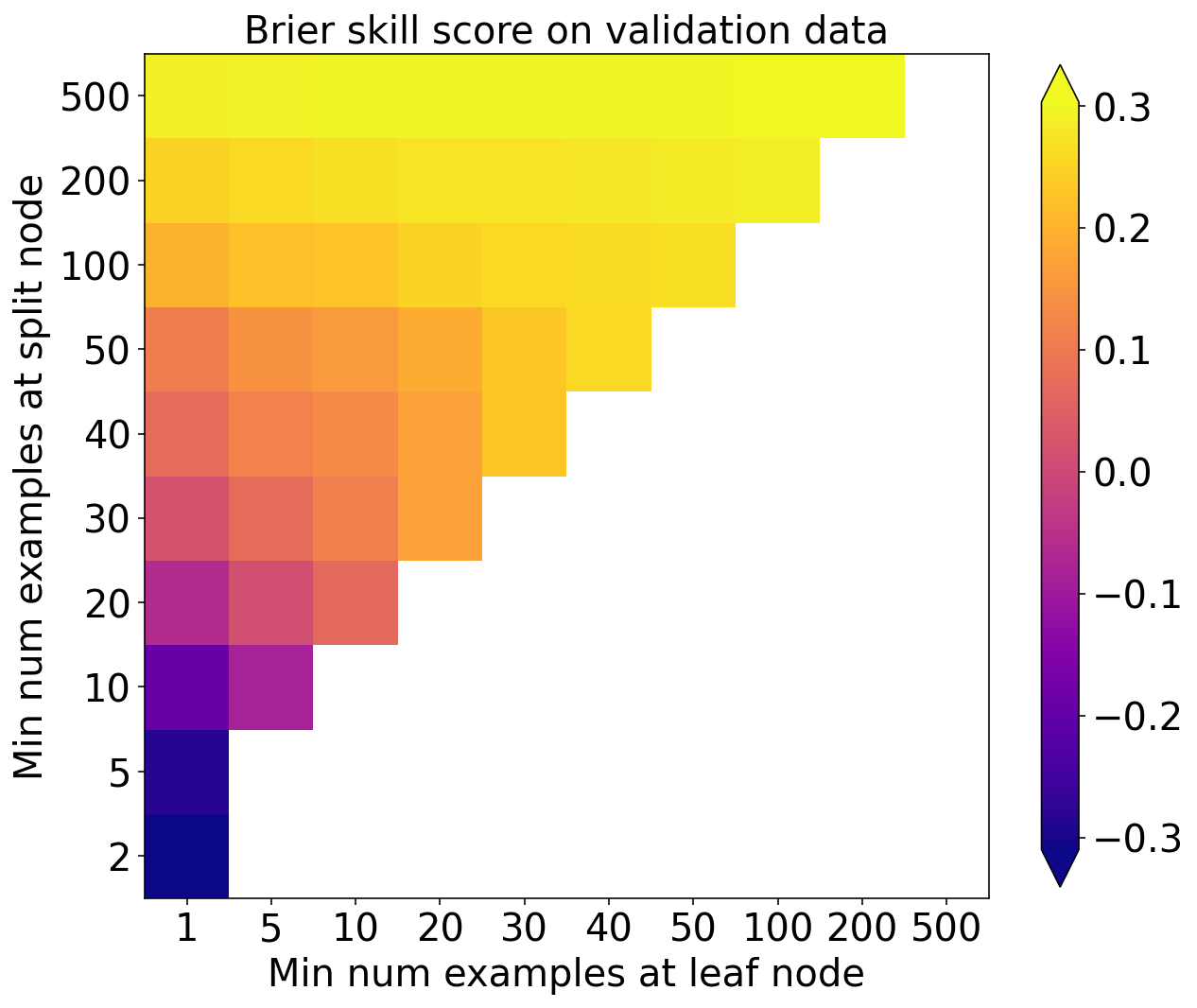
Brier skill score

plot_scores_2d(
    score_matrix=validation_bss_matrix,
    min_colour_value=np.nanpercentile(validation_bss_matrix, 1.),
    max_colour_value=np.nanpercentile(validation_bss_matrix, 99.),
    x_tick_labels=min_per_leaf_values,
    y_tick_labels=min_per_split_values
)

pyplot.xlabel('Min num examples at leaf node')
pyplot.ylabel('Min num examples at split node')
pyplot.title('Brier skill score on validation data')
pyplot.show()

选择

下一个单元格执行超参数实验的第 4 步（选择模型）。

选择 BSS 最大的模型作为最佳模型

best_linear_index = np.nanargmax(np.ravel(validation_bss_matrix))

best_split_index, best_leaf_index = np.unravel_index(
    best_linear_index, 
    validation_bss_matrix.shape
)

best_min_examples_per_split = min_per_split_values[best_split_index]
best_min_examples_per_leaf = min_per_leaf_values[best_leaf_index]
best_validation_bss = np.nanmax(validation_bss_matrix)

print(
    f'Best validation BSS = {best_validation_bss:.3f}\n'
    f'corresponding min examples per split node = {best_min_examples_per_split}\n'
    f'min examples per leaf node = {best_min_examples_per_leaf}'
)

Best validation BSS = 0.304
corresponding min examples per split node = 500
min examples per leaf node = 200

使用超参数构建并训练模型

final_model = setup_classification_tree(
    min_examples_at_split=best_min_examples_per_split,
    min_examples_at_leaf=best_min_examples_per_leaf
)

_ = train_classification_tree(
    model=final_model,
    training_predictor_table=training_predictor_table,
    training_target_table=training_target_table
)

在测试集上预测

testing_predictions = final_model.predict_proba(
    testing_predictor_table.values
)[:, 1]
training_event_frequency = np.mean(
    training_target_table[BINARIZED_TARGET_NAME].values
)

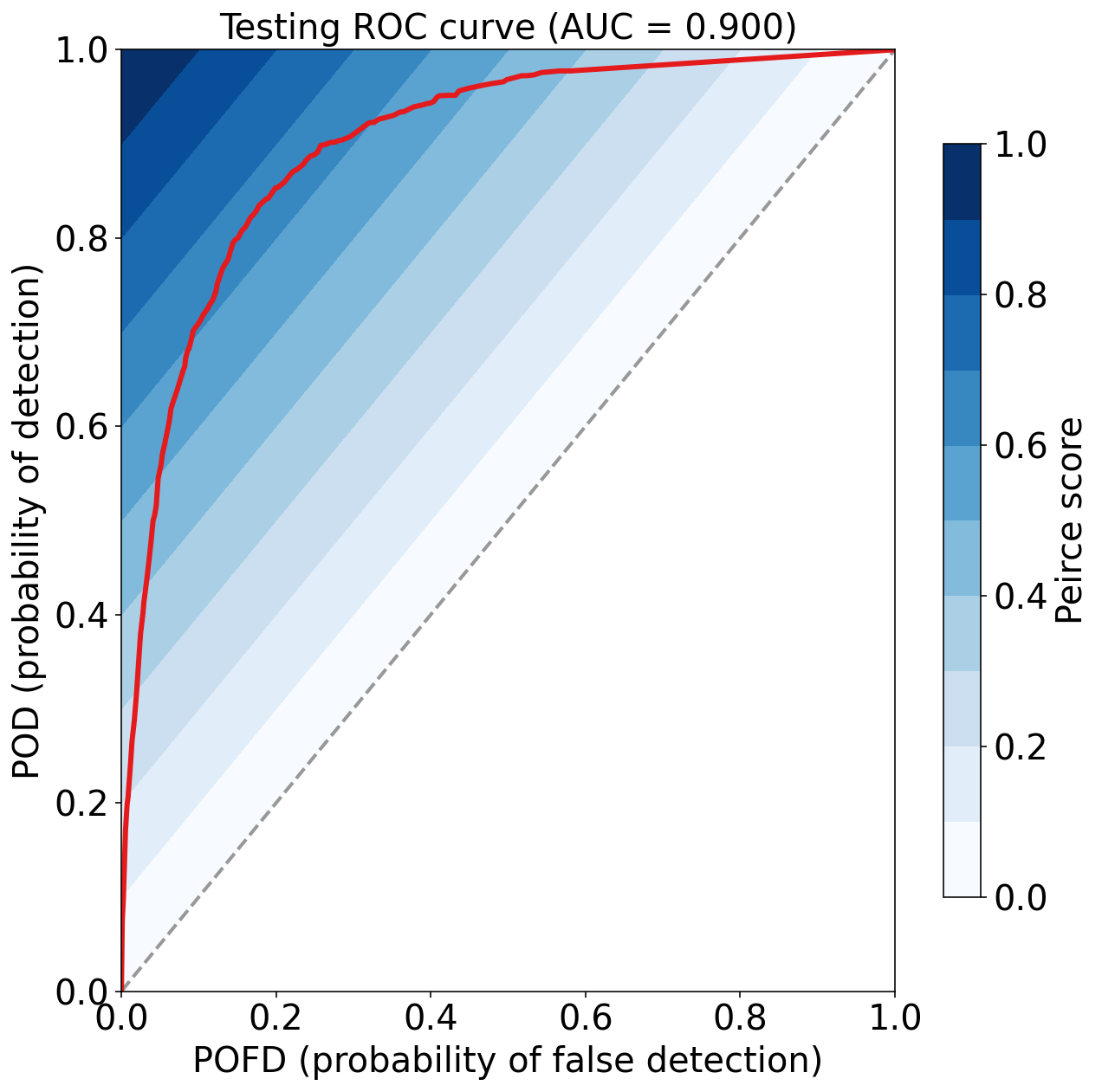
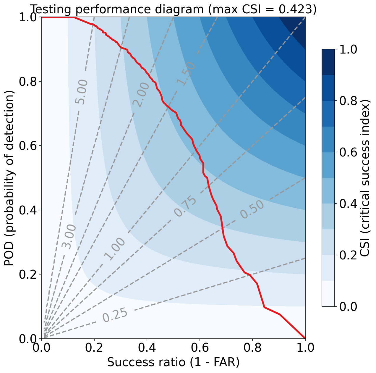
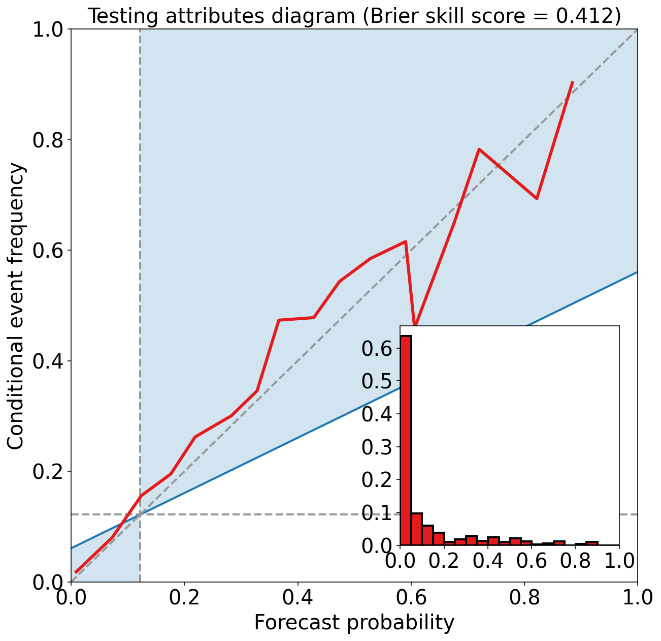
评估在测试集上的性能

_ = eval_binary_classifn(
    observed_labels=testing_target_table[BINARIZED_TARGET_NAME].values,
    forecast_probabilities=testing_predictions,
    training_event_frequency=training_event_frequency,
    create_plots=True, 
    verbose=True, 
    dataset_name='testing'
)

Testing Max Peirce score (POD - POFD) = 0.657
Testing AUC (area under ROC curve) = 0.900
Testing Max CSI (critical success index) = 0.423
Testing Brier score = 0.053
Testing Brier skill score (improvement over climatology) = 0.412

练习

基于第一个超参数实验，编写自己的超参数实验（使用不同的 N_{b}^{min} 和 N_{l}^{min} 集合）。查看是否可以找到在验证数据上更有效的组合。如果找到在验证数据上更有效的组合，请查看它在测试数据上是否也更好。如果不是，则 N_{b}^{min} 和 N_{l}^{min} 在验证集上过拟合。