预测雷暴旋转的基础机器学习：分类 - 性能图

August 19, 2020 (最后修改: August 22, 2021)

本文翻译自 AMS 机器学习 Python 教程，并有部分修改。
Lagerquist, R., and D.J. Gagne II, 2019: “Basic machine learning for predicting thunderstorm rotation: Python tutorial”. https://github.com/djgagne/ams-ml-python-course/blob/master/module_2/ML_Short_Course_Module_2_Basic.ipynb.

本文接上一篇文章，介绍如何绘制性能图 (Performance diagram) 评估二元分类问题。

《预测雷暴旋转的基础机器学习：分类 - ROC 曲线》

性能图

引自
https://www.cawcr.gov.au/projects/verification
https://www.cawcr.gov.au/projects/verification/Roebber/PerformanceDiagram.html

Performance Diagram

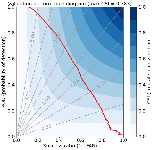
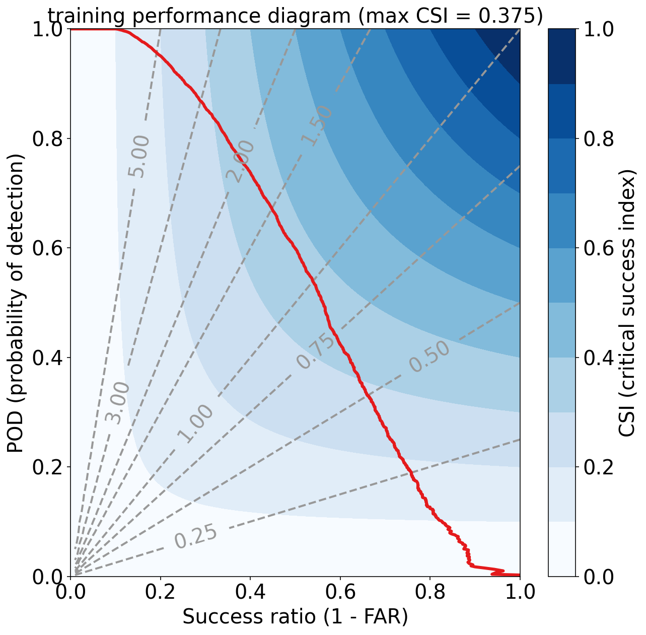
验证数据集上的性能图如下所示

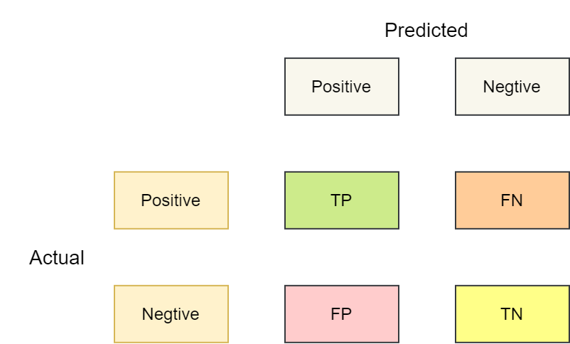
混淆矩阵

二分类问题的混淆矩阵

POD

真阳率

Probability of detection (hit rate)，POD

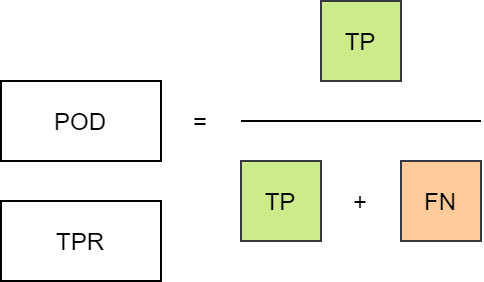
回答如下问题：有多少观察到"是"的事件被正确预测？

范围：0 到 1

完美分数：1

特性：

对 hits (TP) 敏感，但忽略 false alarm (FP)。对事件的气候频率非常敏感。适用于罕见事件。可以通过发布更多“是”预测来增加 hits 次数，从而人为地加以改进。应与 false alarm ratio 结合使用。 POD 还是广泛用于概率预测的Relative Operating Characteristic (ROC) 的重要组成部分。

SR

False alarm ratio, FAR

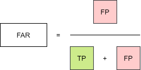
回答如下问题：预测"是"事件中，哪些部分实际上未发生（即误报）？

范围：0 到 1

完美分数：0

特性：

对 false alarm (FP) 敏感，但忽略 miss (FN)。对事件的气候频率非常敏感。应与 POD 结合使用。

Success ratio，SR

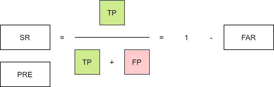
回答如下问题：预测为"是"的事件中哪些部分观测也是“是”？

范围：0 到 1

完美分数：1

特性：

给出有关观察到的事件的可能性的信息（假设已被预测）。它对 false alarm (FP) 很敏感，但忽略 miss (FN)。 SR 等于 1-FAR。在分类性能图 (categorical performance diagram) 中，相对于 SR 绘制了 POD。

CSI

Threat score (TS)，Critical success index (CSI)

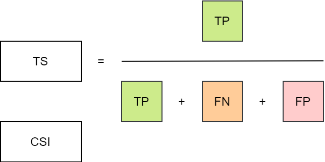
回答如下问题：预测的“是”事件与观察到的“是”事件对应得如何？

范围：0 到 1，0 表示没有技巧

完美分数：0

特性：

测量正确预测的观测和/或预测事件的比例。在不考虑真反例的情况下，可以被当成精确度，也就是说，TS 仅关注有计数的预测。对 hits (TP) 敏感，对 misses (FN) 和 false alarms (FP) 都会造成惩罚。不区分预测误差的来源。取决于事件的气候频率（罕见事件的评分较低），因为某些 hits 可能纯粹是由于随机机会而发生的。

frequency bias

Bias score, frequency bias

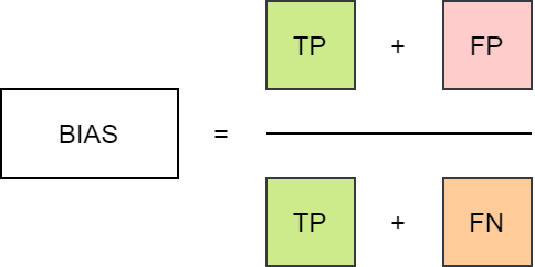
回答如下问题：“是”事件的预测频率与观察到的“是”事件的频率相比如何？

范围：0 到正无穷大

完美分数：1

特性：

测量预测事件的频率与观察到的事件的频率之比。指示预测系统是倾向于发生低预测 (BIAS < 1) 还是发生高预测 (BIAS > 1) 事件。不衡量预测与观测值的对应程度，仅衡量相对频率。

Performance Diagram

在概念上类似于 Taylor diagram 的方法中，有可能利用二分预测性能的四个度量之间的几何关系：probability of detection (POD)，false alarm ratio 或与其相反，success ratio (SR)，bias 和 critical success index (CSI；也称为 threat score，即 TS）。 Roebber（2009）给出了该图的推导细节。

对于良好的预测，POD，SR，bias 和 CSI 趋于一致，因此，完美的预测位于图表的右上方。特定方向的偏差将指示 POD 和 SR 的相对差异，并因此指示 bias 和 CSI。因此，可以立即看到性能差异。准确度的最佳提高是通过沿 45 度移动来实现的，也就是说，通过同时增加检测和减少误报来保持无偏的预测。通过相对于参考预测（气候，持续性或任何其他所需基准）绘制预测质量度量来评估技能。

采样变异性的影响是使用一种重采样的形式来估计的，该替换具有从验证数据中进行 bootstrap 替换。 SR 和 POD 的第 95 个百分位范围被绘制为围绕验证点的“十字线”，并且同时显示了 bias 和 CSI 的变化。使用观察和预测的“是”和“否”条目（即边际频率）的采样频率创建了与原始大小相同的 1000 个新样本，并从这些“气候”样本中计算了第 25 和第 975 精度度量，产生第 95 个百分位范围。

在示例图中，来自Roebber el al.(2003) 的大雪密度和小雪密度验证数据（分别为实心蓝色正方形和圆形）以及相应的采样频率（分别为空心蓝色正方形和圆形）。还显示了 Fowle 和 Roebber (2003)（红色三角形）对流发生的 48 小时预报验证。

参考

Fowle, M.A. and P.J. Roebber, 2003: Short-range (0-48 h) numerical prediction of convective occurrence, mode, and location. Wea. Forecasting, 18, 782-794.

Roebber, P.J., 2009: Visualizing multiple measures of forecast quality. Wea. Forecasting, 24, 601-608.

Roebber, P.J., S.L. Breuning, D.M. Schultz, and J.V. Cortinas, Jr., 2003: Improving snowfall forecasting by diagnosing snow density. Wea. Forecasting, 18, 264-287.

计算性能图数据

get_points_in_perf_diagram 为性能图计算点，返回

真正例率（TPR）
查准率（PRE）

def get_points_in_perf_diagram(
    observed_labels: np.ndarray, 
    forecast_probabilities: np.ndarray,
) -> (np.ndarray, np.ndarray): 
    # 验证数据范围
    assert np.all(np.logical_or(
        observed_labels == 0, observed_labels == 1
    ))

    assert np.all(np.logical_and(
        forecast_probabilities >= 0, forecast_probabilities <= 1
    ))
    
    observed_labels = observed_labels.astype(int)
    binarization_thresholds = np.linspace(
        0, 1, 
        num=1001, 
        dtype=float
    )

    num_thresholds = len(binarization_thresholds)
    pod_by_threshold = np.full(num_thresholds, np.nan)
    success_ratio_by_threshold = np.full(num_thresholds, np.nan)

    for k in range(num_thresholds):
        these_forecast_labels = (
            forecast_probabilities >= binarization_thresholds[k]
        ).astype(int)
        
        # 真阳性 TP
        this_num_hits = np.sum(np.logical_and(
            these_forecast_labels == 1, observed_labels == 1
        ))
        
        # 假阳性 FP
        this_num_false_alarms = np.sum(np.logical_and(
            these_forecast_labels == 1, observed_labels == 0
        ))
        
        # 假阴性 FN
        this_num_misses = np.sum(np.logical_and(
            these_forecast_labels == 0, observed_labels == 1
        ))

        try:
            # 真阳率 TPR = TP / (TP + FN)
            pod_by_threshold[k] = (
                float(this_num_hits) / (this_num_hits + this_num_misses)
            )
        except ZeroDivisionError:
            pass

        try:
            # 精度 PRE = TP / (TP + FP)
            success_ratio_by_threshold[k] = (
                float(this_num_hits) / (this_num_hits + this_num_false_alarms)
            )
        except ZeroDivisionError:
            pass

    pod_by_threshold = np.array([1.] + pod_by_threshold.tolist() + [0.])
    success_ratio_by_threshold = np.array(
        [0.] + success_ratio_by_threshold.tolist() + [1.]
    )

    return pod_by_threshold, success_ratio_by_threshold

绘制性能图

plot_performance_diagram 绘制性能图

def plot_performance_diagram(
    observed_labels, 
    forecast_probabilities,
    line_colour=np.array([228, 26, 28], dtype=float) / 255, 
    line_width=3,
    bias_line_colour=np.full(3, 152. / 255),
    bias_line_width=2, 
    axes_object=None
):    
    # 获取真阳率（TPR）和精度（PRE）
    pod_by_threshold, success_ratio_by_threshold = get_points_in_perf_diagram(
        observed_labels=observed_labels,
        forecast_probabilities=forecast_probabilities
    )

    if axes_object is None:
        _, axes_object = pyplot.subplots(
            1, 1, 
            figsize=(10, 10)
        )
    # 创建 精度 / 真阳率 坐标网格
    success_ratio_matrix, pod_matrix = _get_sr_pod_grid()
    
    # CSI
    csi_matrix = _csi_from_sr_and_pod(
        success_ratio_matrix, 
        pod_matrix
    )
    
    # 频率偏差
    frequency_bias_matrix = _bias_from_sr_and_pod(
        success_ratio_matrix, 
        pod_matrix
    )

    this_colour_map_object, this_colour_norm_object = _get_csi_colour_scheme()
    
    # 绘制 CSI 的填充图
    pyplot.contourf(
        success_ratio_matrix, 
        pod_matrix, 
        csi_matrix, 
        np.linspace(0, 1, num=11, dtype=float),
        cmap=this_colour_map_object, 
        norm=this_colour_norm_object, 
        vmin=0.,
        vmax=1., 
        axes=axes_object
    )
    
    # 为 CSI 填充图添加颜色条
    colour_bar_object = _add_colour_bar(
        axes_object=axes_object, 
        colour_map_object=this_colour_map_object,
        colour_norm_object=this_colour_norm_object,
        values_to_colour=csi_matrix, 
        min_colour_value=0.,
        max_colour_value=1., 
        orientation_string='vertical',
        extend_min=False, 
        extend_max=False
    )
    colour_bar_object.set_label('CSI (critical success index)')
    
    LEVELS_FOR_BIAS_CONTOURS = np.array([0.25, 0.5, 0.75, 1., 1.5, 2., 3., 5.])

    bias_colour_tuple = ()
    for _ in range(len(LEVELS_FOR_BIAS_CONTOURS)):
        bias_colour_tuple += (bias_line_colour,)
    
    # 绘制频率偏差等值线（虚线）
    bias_contour_object = pyplot.contour(
        success_ratio_matrix, 
        pod_matrix, 
        frequency_bias_matrix,
        LEVELS_FOR_BIAS_CONTOURS, 
        colors=bias_colour_tuple,
        linewidths=bias_line_width, 
        linestyles='dashed', 
        axes=axes_object,
    )
    # 为频率偏差等值线添加标签
    pyplot.clabel(
        bias_contour_object, 
        inline=True, 
        inline_spacing=10,
        fmt='%.2f', 
        fontsize=20,
    )

    nan_flags = np.logical_or(
        np.isnan(success_ratio_by_threshold), 
        np.isnan(pod_by_threshold)
    )
    
    # 绘制 精度 / 真阳率 线图
    if not np.all(nan_flags):
        real_indices = np.where(np.invert(nan_flags))[0]
        axes_object.plot(
            success_ratio_by_threshold[real_indices],
            pod_by_threshold[real_indices], 
            color=line_colour,
            linestyle='solid', 
            linewidth=line_width
        )

    axes_object.set_xlabel('Success ratio (1 - FAR)')
    axes_object.set_ylabel('POD (probability of detection)')
    axes_object.set_xlim(0., 1.)
    axes_object.set_ylim(0., 1.)

    return pod_by_threshold, success_ratio_by_threshold

_get_sr_pod_grid 创建 SR-POD 坐标网格（success ratio / probability of detection，精度 / 真阳率）

def _get_sr_pod_grid(success_ratio_spacing=0.01, pod_spacing=0.01):
    num_success_ratios = 1 + int(np.ceil(1. / success_ratio_spacing))
    num_pod_values = 1 + int(np.ceil(1. / pod_spacing))

    unique_success_ratios = np.linspace(0., 1., num=num_success_ratios)
    unique_pod_values = np.linspace(0., 1., num=num_pod_values)[::-1]
    return np.meshgrid(unique_success_ratios, unique_pod_values)

_csi_from_sr_and_pod 函数计算 CSI（critical success index，临界成功指数）

def _csi_from_sr_and_pod(
    success_ratio_array: np.ndarray, 
    pod_array: np.ndarray
) -> np.ndarray:
    return (success_ratio_array ** -1 + pod_array ** -1 - 1.) ** -1

_bias_from_sr_and_pod 函数根据精度和真阳率计算频率偏差

def _bias_from_sr_and_pod(
    success_ratio_array, 
    pod_array
):
    return pod_array / success_ratio_array

_get_csi_colour_scheme 函数为 CSI 指数生成色表

def _get_csi_colour_scheme():
    LEVELS_FOR_CSI_CONTOURS = np.linspace(0, 1, num=11, dtype=float)

    this_colour_map_object = pyplot.cm.Blues
    this_colour_norm_object = matplotlib.colors.BoundaryNorm(
        LEVELS_FOR_CSI_CONTOURS, 
        this_colour_map_object.N
    )

    rgba_matrix = this_colour_map_object(
        this_colour_norm_object(
            LEVELS_FOR_CSI_CONTOURS
        )
    )
    colour_list = [
        rgba_matrix[i, ..., :-1] for i in range(rgba_matrix.shape[0])
    ]

    colour_map_object = matplotlib.colors.ListedColormap(colour_list)
    colour_map_object.set_under(np.array([1, 1, 1]))
    
    colour_norm_object = matplotlib.colors.BoundaryNorm(
        LEVELS_FOR_CSI_CONTOURS, 
        colour_map_object.N
    )

    return colour_map_object, colour_norm_object

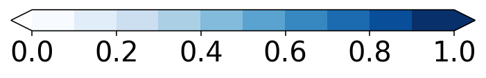
绘制 CSI 填充图的颜色条

colour_map_object, colour_norm_object = _get_csi_colour_scheme()
scalar_mappable_object = pyplot.cm.ScalarMappable(
    cmap=colour_map_object, 
    norm=colour_norm_object
)
pyplot.colorbar( 
    mappable=scalar_mappable_object,
    orientation='horizontal', 
    pad=0.075, 
    extend='both',
    shrink=1
)
pyplot.gca().set_visible(False)

示例

dataset_name = "training"

pod_by_threshold, success_ratio_by_threshold = (
    get_points_in_perf_diagram(
        observed_labels=training_target_table["strong_future_rotation_flag"].values,
        forecast_probabilities=training_probabilities
    )
)
    
csi_by_threshold = (
    (pod_by_threshold ** -1 + success_ratio_by_threshold ** -1 - 1) ** -1
)
max_csi = np.nanmax(csi_by_threshold)

_, axes_object = pyplot.subplots(
    1, 1, 
    figsize=(
        10, 
        10
    )
)

plot_performance_diagram(
    observed_labels=training_target_table["strong_future_rotation_flag"].values,
    forecast_probabilities=training_probabilities,
    axes_object=axes_object
)

pyplot.title(
    f'{dataset_name} performance diagram '
    f'(max CSI = {max_csi:.3f})'
)
pyplot.show()