AMS机器学习课程:预测雷暴旋转的基础机器学习 - 数据
本文翻译自 AMS 机器学习 Python 教程,并有部分修改。
Lagerquist, R., and D.J. Gagne II, 2019: “Basic machine learning for predicting thunderstorm rotation: Python tutorial”. https://github.com/djgagne/ams-ml-python-course/blob/master/module_2/ML_Short_Course_Module_2_Basic.ipynb.
该模块使用基本的机器学习模型 ———— 线性回归,逻辑回归,决策树,随机森林和梯度增强树 ———— 来预测来自 NCAR convection-allowing ensemble 的数值模拟中未来的雷暴旋转(Schwartz et al. 2015)。
请按以下方式引用笔记本。
Lagerquist, R., and D.J. Gagne II, 2019: “Basic machine learning for predicting thunderstorm rotation: Python tutorial”. https://github.com/djgagne/ams-ml-python-course/blob/master/module_2/ML_Short_Course_Module_2_Basic.ipynb.
注:本文使用的数据需要额外下载,请浏览《AMS机器学习课程:数据分析与预处理》获取更多信息。
参考文献
本笔记本引用了下面列出的一些出版物。
Chisholm, D., J. Ball, K. Veigas, and P. Luty, 1968: “The diagnosis of upper-level humidity.” Journal of Applied Meteorology, 7 (4), 613-619.
Hsu, W., and A. Murphy, 1986: “The attributes diagram: A geometrical framework for assessing the quality of probability forecasts.” International Journal of Forecasting, 2, 285–293, https://doi.org/10.1016/0169-2070(86)90048-8.
McGovern, A., D. Gagne II, J. Basara, T. Hamill, and D. Margolin, 2015: “Solar energy prediction: An international contest to initiate interdisciplinary research on compelling meteorological problems.” Bulletin of the American Meteorological Society, 96 (8), 1388-1395.
Metz, C., 1978: “Basic principles of ROC analysis.” Seminars in Nuclear Medicine, 8, 283–298, https://doi.org/10.1016/S0001-2998(78)80014-2.
Quinlan, J., 1986: “Induction of decision trees.” Machine Learning, 1 (1), 81–106.
Roebber, P., 2009: “Visualizing multiple measures of forecast quality.” Weather and Forecasting, 24, 601-608, https://doi.org/10.1175/2008WAF2222159.1.
Schwartz, C., G. Romine, M. Weisman, R. Sobash, K. Fossell, K. Manning, and S. Trier, 2015: “A real-time convection-allowing ensemble prediction system initialized by mesoscale ensemble Kalman filter analyses.” Weather and Forecasting, 30 (5), 1158-1181.
安装
要使用此笔记本,您将需要 Python 3.6 和以下软件包。
- scipy
- TensorFlow
- Keras
- scikit-image
- netCDF4
- pyproj
- scikit-learn
- opencv-python
- matplotlib
- shapely
- geopy
- metpy
- descartes
注:笔者使用 Python 3.7
导入
下一个单元格将导入此笔记本将使用的所有库。 如果笔记本在任何地方崩溃,则可能在此处。
import copy
import warnings
import pathlib
import glob
import typing

import matplotlib.pyplot as pyplot
import numpy as np
import pandas as pd
from tqdm import tqdm
from sklearn import linear_model

MODULE2_DIR_NAME = '.'
SHORT_COURSE_DIR_NAME = '..'
utils 库
原始项目将数据处理和模型训练等相关函数封装到 utils 包中,下面的截图来自 VSCode:
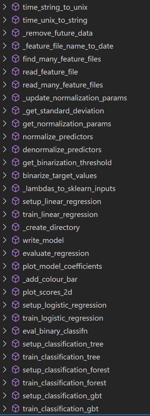
译者注:本文不会直接调用 utils 包,而是介绍示例中使用到的所有函数源代码。
过拟合
谈论机器学习就不能不谈论过拟合。 当模型在训练数据上表现良好但不能很好地推广到新数据时,就会发生过拟合。 这通常在以下情况下发生:
- 训练集太小
- 训练集包含不适当的预测变量
- 训练集不能代表真实世界
不适当的预测变量示例:
- 使用风暴 ID 预测龙卷风
- 使用病人 ID 预测疾病
- 更一般的情况是使用与目标现象没有物理关系的变量
非代表性训练数据的示例:
- 标签分布不同。例如训练集包含 50% 的龙卷风暴,但现实世界中只有小于 1% 的风暴是龙卷
- 不同级别的数据质量。例如,对已存档的雷达数据进行训练,但应用于实时数据
您可以通过不犯这些错误来减轻过拟合的情况。 但是,这些属性(预测变量的适当性,训练数据的代表性等)并不总是很清楚。
同样,许多其他因素也可能导致过度拟合。
因此,您还需要具有诊断过拟合的能力。
通常,这可以通过将数据分为3个分区来完成:训练集,验证集和测试集。
训练集,验证集和测试集
训练集的角色:训练模型。例如,调整线性回归或神经网络中的权重,调整决策树中的决策边界等。
验证集的角色:选择最佳的超参数(不由训练调整的参数)。 例如学习率,迭代次数,神经网络中的层数
测试集的角色:根据独立数据评估所选模型。 所选模型是对验证数据表现最佳的模型。 定义“最佳”的方法有很多(最低均方误差,最小交叉熵,ROC 曲线下的最大面积等)。
训练,验证和测试(TV&T)数据集应在统计上独立。
例如在疾病预测中:
- 如果同一位患者进行了多次组织扫描,则它们应该都在同一组中。
- 同一家族中的多个患者也应位于同一组中。
在风暴灾害预测中:
- 如果同一风暴有多个雷达扫描,则它们应全部位于同一集合中。
- 相关风暴(例如,同一 MCS 的一部分)也应位于同一集合中。
在通用天气预测中:
- 数据应无时间自相关。
对于风暴规模的现象,在每对数据集之间留出一天的间隔可能就足够了。 对于天气尺度现象,每对数据集之间可能需要一个星期的间隔。
- 如果在一个区域上进行训练并应用于另一区域,则数据应没有空间自相关。
例如,假设您正在针对北美的模型进行培训,但实时应用于非洲。 数据集(TV&T)应包含北美在空间上不重叠的部分。 当您在尚未用于训练/验证模型的北美部分进行测试时,希望可以为您提供对非洲性能的合理估计,而非洲也尚未用于训练/验证模型。
查找输入文件
下一个单元查找训练(2010-2014),验证(2015)和测试(2016-2017)期间的输入文件。
使用到的函数
feature_file_name_to_date
feature_file_name_to_date 函数从 CSV 文件名中提取日期
def feature_file_name_to_date(csv_file_name: str) -> pd.Timestamp:
    file_name = pathlib.Path(csv_file_name).name
    date_string = file_name.replace(
        'track_step_NCARSTORM_d01_', ''
    ).replace('-0000.csv', '')

    return pd.to_datetime(date_string, format='%Y%m%d')

feature_file_name_to_date(
    "../data/track_data_ncar_ams_3km_csv_small/track_step_NCARSTORM_d01_20110308-0000.csv"
)
Timestamp('2011-03-08 00:00:00')
find_many_feature_files
find_many_feature_files 函数根据给定的日志范围查找符合条件的 CSV 文件。
def find_many_feature_files(
    first_date: str or pd.Timestamp,
    last_date: str or pd.Timestamp,
    feature_dir_name="../data/track_data_ncar_ams_3km_csv_small"
) -> typing.List:
    first_time = pd.to_datetime(
        first_date
    )
    last_time = pd.to_datetime(
        last_date
    )

    DATE_FORMAT = '%Y%m%d'
    DATE_FORMAT_REGEX = '[0-9][0-9][0-9][0-9][0-1][0-9][0-3][0-9]'
    csv_file_pattern = f'{feature_dir_name}/track_step_NCARSTORM_d01_{DATE_FORMAT_REGEX}-0000.csv'
    csv_file_names = glob.glob(csv_file_pattern)
    csv_file_names.sort()

    file_dates = np.array([
        feature_file_name_to_date(f) for f in csv_file_names
    ])

    good_indices = np.where(np.logical_and(
        file_dates >= first_time,
        file_dates <= last_time
    ))[0]

    return [csv_file_names[k] for k in good_indices]
获取文件列表
获取训练集的文件列表
training_file_names = find_many_feature_files(
    first_date="2010-01-01",
    last_date="2014-12-31",
)
training_file_names[:4]
['../data/track_data_ncar_ams_3km_csv_small\\track_step_NCARSTORM_d01_20101024-0000.csv',
 '../data/track_data_ncar_ams_3km_csv_small\\track_step_NCARSTORM_d01_20101122-0000.csv',
 '../data/track_data_ncar_ams_3km_csv_small\\track_step_NCARSTORM_d01_20110201-0000.csv',
 '../data/track_data_ncar_ams_3km_csv_small\\track_step_NCARSTORM_d01_20110308-0000.csv']
获取验证集的文件列表
validation_file_names = find_many_feature_files(
    first_date="20150101",
    last_date="20151231",
)
validation_file_names[-4:]
['../data/track_data_ncar_ams_3km_csv_small\\track_step_NCARSTORM_d01_20150706-0000.csv',
 '../data/track_data_ncar_ams_3km_csv_small\\track_step_NCARSTORM_d01_20150712-0000.csv',
 '../data/track_data_ncar_ams_3km_csv_small\\track_step_NCARSTORM_d01_20151031-0000.csv',
 '../data/track_data_ncar_ams_3km_csv_small\\track_step_NCARSTORM_d01_20151227-0000.csv']
获取测试集的文件列表
testing_file_names = find_many_feature_files(
    first_date="20160101",
    last_date="20171231",
)
testing_file_names[:5]
['../data/track_data_ncar_ams_3km_csv_small\\track_step_NCARSTORM_d01_20160224-0000.csv',
 '../data/track_data_ncar_ams_3km_csv_small\\track_step_NCARSTORM_d01_20160323-0000.csv',
 '../data/track_data_ncar_ams_3km_csv_small\\track_step_NCARSTORM_d01_20160401-0000.csv',
 '../data/track_data_ncar_ams_3km_csv_small\\track_step_NCARSTORM_d01_20160415-0000.csv',
 '../data/track_data_ncar_ams_3km_csv_small\\track_step_NCARSTORM_d01_20160429-0000.csv']
读取数据
下一个单元格读取训练、验证和测试数据,并浏览一个文件的内容。
使用到的函数
变量名
# 元信息列,不需要
METADATA_COLUMNS = [
    'Step_ID', 'Track_ID', 'Ensemble_Name', 'Ensemble_Member', 'Run_Date',
    'Valid_Date', 'Forecast_Hour', 'Valid_Hour_UTC'
]

# 不需要的列
EXTRANEOUS_COLUMNS = [
    'Duration', 'Centroid_Lon', 'Centroid_Lat', 'Centroid_X', 'Centroid_Y',
    'Storm_Motion_U', 'Storm_Motion_V', 'Matched', 'Max_Hail_Size',
    'Num_Matches', 'Shape', 'Location', 'Scale'
]

# 目标列
TARGET_NAME = 'RVORT1_MAX-future_max'
_remove_future_data
_remove_future_data 函数删除 pd.DataFrame 中列名中有 future 的列
def _remove_future_data(predictor_table):
    predictor_names = list(predictor_table)
    columns_to_remove = [p for p in predictor_names if 'future' in p]

    return predictor_table.drop(
        columns_to_remove,
        axis=1,
        inplace=False
    )
说明:
axis=1表示删除列标签(默认值是axis=0,表示删除索引标签)inplace=False表示返回新的对象,而inplace=True则修改当前的对象
read_feature_file
read_feature_file 函数读取 CSV 文件,返回三个表格,每行代表一个风暴
- 元信息表格
- 预测变量表格
- 目标变量表格
def read_feature_file(csv_file_name):
    predictor_table = pd.read_csv(
        csv_file_name,
        header=0,
        sep=','
    )

    # 删掉不需要的列
    predictor_table.drop(
        EXTRANEOUS_COLUMNS,
        axis=1,
        inplace=True
    )

    # 元信息表格
    metadata_table = predictor_table[METADATA_COLUMNS]
    predictor_table.drop(
        METADATA_COLUMNS,
        axis=1,
        inplace=True
    )

    # 目标表格
    target_table = predictor_table[[TARGET_NAME]]
    predictor_table.drop(
        [TARGET_NAME],
        axis=1,
        inplace=True
    )

    predictor_table = _remove_future_data(predictor_table)

    return metadata_table, predictor_table, target_table
示例
metadata_table, predictor_table, target_table = read_feature_file(
    "../data/track_data_ncar_ams_3km_csv_small/track_step_NCARSTORM_d01_20110308-0000.csv"
)
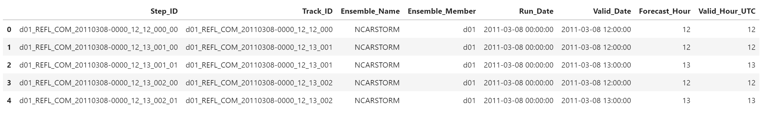
查看返回的三个 pandas.DataFrame 对象
metadata_table.head()
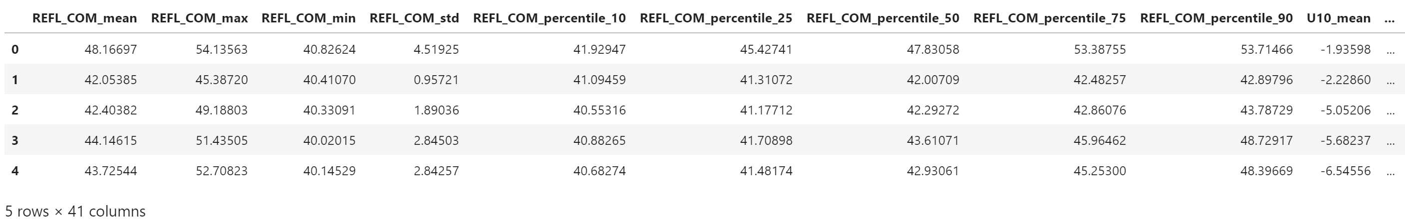
predictor_table.head()
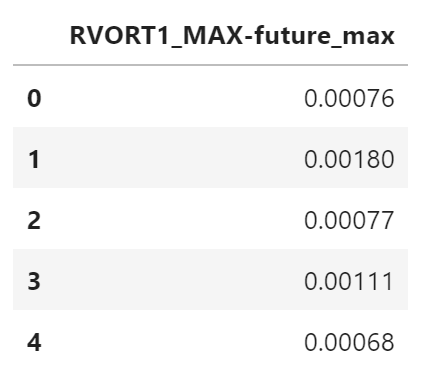
target_table.head()
read_many_feature_files
read_many_feature_files 函数批量读取 CSV 文件
def read_many_feature_files(csv_file_names):
    num_files = len(csv_file_names)
    list_of_metadata_tables = [pd.DataFrame()] * num_files
    list_of_predictor_tables = [pd.DataFrame()] * num_files
    list_of_target_tables = [pd.DataFrame()] * num_files

    for i in tqdm(range(num_files)):
        (
            list_of_metadata_tables[i],
            list_of_predictor_tables[i],
            list_of_target_tables[i]
        ) = read_feature_file(csv_file_names[i])

        if i == 0:
            continue

        list_of_metadata_tables[i] = list_of_metadata_tables[i].align(
            list_of_metadata_tables[0],
            axis=1
        )[0]

        list_of_predictor_tables[i] = list_of_predictor_tables[i].align(
            list_of_predictor_tables[0],
            axis=1
        )[0]

        list_of_target_tables[i] = list_of_target_tables[i].align(
            list_of_target_tables[0],
            axis=1
        )[0]

    metadata_table = pd.concat(
        list_of_metadata_tables,
        axis=0,
        ignore_index=True
    )
    predictor_table = pd.concat(
        list_of_predictor_tables,
        axis=0,
        ignore_index=True
    )
    target_table = pd.concat(
        list_of_target_tables,
        axis=0,
        ignore_index=True
    )

    return (
        metadata_table,
        predictor_table,
        target_table,
    )
说明:
pandas.DataFrame.align 函数用于对齐数据。
axis=1表示对齐列
pandas.concat 用于连接数据
axis=0表示沿 index 连接,默认值ignore_index表示忽略 index,返回的数据重新创建顺序索引
加载数据
训练数据集
(
    training_metadata_table,
    training_predictor_table_denorm,
    training_target_table
) = read_many_feature_files(training_file_names)
验证数据集
(
    validation_metadata_table,
    validation_predictor_table_denorm,
    validation_target_table
) = read_many_feature_files(validation_file_names)
测试数据集
(
    testing_metadata_table,
    testing_predictor_table_denorm,
    testing_target_table
) = read_many_feature_files(testing_file_names)
查看数据内容
元数据表格中的变量
list(training_metadata_table)
['Step_ID',
 'Track_ID',
 'Ensemble_Name',
 'Ensemble_Member',
 'Run_Date',
 'Valid_Date',
 'Forecast_Hour',
 'Valid_Hour_UTC']
预测变量表格中的变量
list(training_predictor_table_denorm)
['REFL_COM_mean',
 'REFL_COM_max',
 'REFL_COM_min',
 'REFL_COM_std',
 'REFL_COM_percentile_10',
 'REFL_COM_percentile_25',
 'REFL_COM_percentile_50',
 'REFL_COM_percentile_75',
 'REFL_COM_percentile_90',
 'U10_mean',
 'U10_max',
 'U10_min',
 'U10_std',
 'U10_percentile_10',
 'U10_percentile_25',
 'U10_percentile_50',
 'U10_percentile_75',
 'U10_percentile_90',
 'V10_mean',
 'V10_max',
 'V10_min',
 'V10_std',
 'V10_percentile_10',
 'V10_percentile_25',
 'V10_percentile_50',
 'V10_percentile_75',
 'V10_percentile_90',
 'T2_mean',
 'T2_max',
 'T2_min',
 'T2_std',
 'T2_percentile_10',
 'T2_percentile_25',
 'T2_percentile_50',
 'T2_percentile_75',
 'T2_percentile_90',
 'area',
 'eccentricity',
 'major_axis_length',
 'minor_axis_length',
 'orientation']
目标变量表格中的变量
list(training_target_table)
['RVORT1_MAX-future_max']
第一个预测变量的名称
first_predictor_name = list(training_predictor_table_denorm)[0]
first_predictor_name
'REFL_COM_mean'
第一个预测变量的样本值
training_predictor_table_denorm[first_predictor_name][:10]
0    42.71822
1    47.09285
2    45.53852
3    44.30976
4    44.64383
5    44.33831
6    45.73259
7    43.69113
8    45.38040
9    47.31104
Name: REFL_COM_mean, dtype: float64
目标变量的名称
target_name = list(training_target_table)[0]
target_name
'RVORT1_MAX-future_max'
目标变量的样本值
training_target_table[target_name][:10]
0    0.00035
1    0.00195
2    0.00241
3    0.00233
4    0.00254
5    0.00174
6    0.00120
7    0.00070
8    0.00050
9    0.00080
Name: RVORT1_MAX-future_max, dtype: float64
标准化
当您有多个不同尺度的预测变量时,应将其标准化。 这样可以确保模型不会忽略较小比例的变量。
例如,如果模型以开尔文为单位的温度和单位为 kg kg^{-1} 的特定湿度进行训练,则它可能会学会强调温度(从 ~180-330 K 变化)而忽略特定湿度( 其范围为 ~0-0.02 kg kg^{-1})。
最常见的标准化方法是 z-score。 每个预测变量使用训练数据的均值和标准差独立转换为 z-score。 验证和测试数据也应标准化,但要使用训练数据的平均值和标准偏差。
问题:为什么使用验证/测试数据来计算均值和标准差(或任何其他数据处理参数)是一个坏主意?
标准化代码
下一个单元格执行以下操作::
- 仅基于训练数据查找每个预测变量的归一化参数(均值和标准差)。
- 使用这些归一化参数对训练,验证和测试数据进行归一化。
- 对训练数据进行反规范化,并确保反规范化的值=原始值(合理性检查)。
使用到的函数
normalize_predictors
normalize_predictors 用于归一化数据,返回归一化后的数据和归一化使用的参数(均值和标准差)
def normalize_predictors(
    predictor_table: pd.DataFrame,
    normalization_dict: typing.Dict or None=None
):
    predictor_names = list(predictor_table)
    num_predictors = len(predictor_names)

    if normalization_dict is None:
        normalization_dict = {}

        for m in range(num_predictors):
            # 计算每列(每个变量)的均值和标准差
            this_mean = np.mean(predictor_table[predictor_names[m]].values)
            this_stdev = np.std(
                predictor_table[predictor_names[m]].values,
                ddof=1,
            )

            # 将计算结果保存到字典对象中
            normalization_dict[predictor_names[m]] = np.array(
                [this_mean, this_stdev]
            )

    for m in range(num_predictors):
        this_mean = normalization_dict[predictor_names[m]][0]
        this_stdev = normalization_dict[predictor_names[m]][1]
        these_norm_values = (
            predictor_table[predictor_names[m]].values - this_mean
        ) / this_stdev

        # 使用归一化后的值代替原有数据
        predictor_table = predictor_table.assign(**{
            predictor_names[m]: these_norm_values
        })

    return predictor_table, normalization_dict
说明:
numpy.std 默认的自由度为 0,上面的函数将自由度设为 1
pandas.DataFrame.assign 设置新的列,如果列已存在则直接替换
denormalize_predictors
denormalize_predictors 用于反归一化,恢复原始的数据值
def denormalize_predictors(
    predictor_table: pd.DataFrame,
    normalization_dict: typing.Dict,
):
    predictor_names = list(predictor_table)
    num_predictors = len(predictor_names)

    for m in range(num_predictors):
        this_mean = normalization_dict[predictor_names[m]][0]
        this_stdev = normalization_dict[predictor_names[m]][1]
        these_denorm_values = (
            this_mean + this_stdev * predictor_table[predictor_names[m]].values
        )

        predictor_table = predictor_table.assign(**{
            predictor_names[m]: these_denorm_values
        })

    return predictor_table
数据转换
第一个变量的前 10 个原始值
predictor_names = list(training_predictor_table_denorm)
training_predictor_table_denorm[predictor_names[0]][:10]
0    42.71822
1    47.09285
2    45.53852
3    44.30976
4    44.64383
5    44.33831
6    45.73259
7    43.69113
8    45.38040
9    47.31104
Name: REFL_COM_mean, dtype: float64
归一化整个输入数据
training_predictor_table, normalization_dict = normalize_predictors(
    predictor_table=copy.deepcopy(training_predictor_table_denorm)
)
第一个变量前 10 个数据归一化后的值
training_predictor_table[predictor_names[0]][:10]
0   -1.036195
1    0.061830
2   -0.328305
3   -0.636721
4   -0.552870
5   -0.629555
6   -0.279593
7   -0.791996
8   -0.367992
9    0.116595
Name: REFL_COM_mean, dtype: float64
从归一化后的数据反推原始数据
training_predictor_table_denorm = denormalize_predictors(
    predictor_table=copy.deepcopy(training_predictor_table),
    normalization_dict=normalization_dict
)
training_predictor_table_denorm[predictor_names[0]][:10]
0    42.71822
1    47.09285
2    45.53852
3    44.30976
4    44.64383
5    44.33831
6    45.73259
7    43.69113
8    45.38040
9    47.31104
Name: REFL_COM_mean, dtype: float64
可以看到,反归一化得到的值与原始数据相同。
下面使用同样的参数归一化验证和测试数据集。
validation_predictor_table, _ = normalize_predictors(
    predictor_table=copy.deepcopy(validation_predictor_table_denorm),
    normalization_dict=normalization_dict,
)

testing_predictor_table, _ = normalize_predictors(
    predictor_table=copy.deepcopy(testing_predictor_table_denorm),
    normalization_dict=normalization_dict,
)
