AMS机器学习课程：数据分析与预处理

July 26, 2020 (最后修改: August 22, 2021)

meteorology/ml

本文翻译自 AMS 机器学习 Python 教程，并有部分修改。

准备

本文来自 djgagne/ams-ml-python-course 项目，请在运行下面代码前执行该项目的 download_data.py 文件下载需要的 csv 文件和 NetCDF 文件。

机器学习途径

大部分机器学习工作流包含 6 个步骤：

探索性分析：加载和可视化数据以了解其分布方式以及不同变量之间的相互关系。
预处理：将您的数据转换为更适合机器学习的形式。
模型训练：使用您的预处理数据优化一个或多个机器学习模型。
模型推断：将机器学习模型应用于训练集之外的数据。
评估：确定您的机器学习模型的执行情况。
解释：提取您的模型从数据中学到的知识。

在本节中，我们将介绍步骤 1 和 2。您将学习教程数据集，对其进行探索，并执行一些预处理任务。

短期课程数据和问题简介

该问题的目标是预测低级别涡流（low-level vorticity）超过特定阈值的概率，给定一个风暴的模拟雷达反射率 > 40 dBZ 和相关的地面风和温度场。

netCDF 数据中的输入要素场

REFL_COM_curr (组合反射率)
U10_curr (10 m 西东风分量，m/s)
V10_curr (10 m 南北风分量，m/s)
T2_curr (2m 温度，开尔文)

预测要素

RVORT1_MAX_future (每小时最大垂直涡流，高于地面 1 公里，每秒速度)

其他值得关注的变量

time：风暴图像的有效时间
i 和 j：来自原始 WRF 模式网格的行和列数组索引
x 和 y：投影坐标（以 m 表示）
masks：显示风暴轮廓的二进制网格。csv 文件中的聚合统计信息仅从蒙版中的正网格点中提取

使用 pandas 和 xarray 读取气象数据文件

首先我们需要导入本节中使用的库，并修改部分设置。

%matplotlib inline
%config InlineBackend.figure_format = 'retina'

import numpy as np
import netCDF4 as nc
import pandas as pd
import xarray as xr

import matplotlib.pyplot as plt
from matplotlib.colors import LogNorm

from scipy.stats import percentileofscore

import cartopy.crs as ccrs
import cartopy.feature as cfeature

import pathlib
import os

xr.set_options(display_style="text");

探索 CSV 文件

查找 CSV 文件

如何查找 CSV 文件并为找到的文件创建排序列表

为此，我们使用 pathlib 库列出指定目录中的所有 *.csv 文件。

# 创建 `pathlib.Path` 对象
path = pathlib.Path("../data/track_data_ncar_ams_3km_csv_small/")

# 查找 `path` 目录下的所有 csv 文件
files = sorted(path.glob("*.csv"))
files[:5]

[WindowsPath('../data/track_data_ncar_ams_3km_csv_small/track_step_NCARSTORM_d01_20101024-0000.csv'),
 WindowsPath('../data/track_data_ncar_ams_3km_csv_small/track_step_NCARSTORM_d01_20101122-0000.csv'),
 WindowsPath('../data/track_data_ncar_ams_3km_csv_small/track_step_NCARSTORM_d01_20110201-0000.csv'),
 WindowsPath('../data/track_data_ncar_ams_3km_csv_small/track_step_NCARSTORM_d01_20110308-0000.csv'),
 WindowsPath('../data/track_data_ncar_ams_3km_csv_small/track_step_NCARSTORM_d01_20110326-0000.csv')]

加载 CSV 文件

如何使用 Pandas 读取 CSV 文件并连接所有内容

下面的方法将所有 csv 文件的内容添加到一个 Python Pandas DataFraome 对象中。我们同时还打印数据的列标签，帮助我们确定哪些 key 可以使用。

df = pd.concat(
    [pd.read_csv(f) for f in files],
    ignore_index=True,
)
for key in df.keys():
    print(key)

Step_ID
Track_ID
Ensemble_Name
Ensemble_Member
Run_Date
Valid_Date
Forecast_Hour
Valid_Hour_UTC
Duration
Centroid_Lon
Centroid_Lat
Centroid_X
Centroid_Y
Storm_Motion_U
Storm_Motion_V
REFL_COM_mean
REFL_COM_max
REFL_COM_min
REFL_COM_std
REFL_COM_percentile_10
REFL_COM_percentile_25
REFL_COM_percentile_50
REFL_COM_percentile_75
REFL_COM_percentile_90
U10_mean
U10_max
U10_min
U10_std
U10_percentile_10
U10_percentile_25
U10_percentile_50
U10_percentile_75
U10_percentile_90
V10_mean
V10_max
V10_min
V10_std
V10_percentile_10
V10_percentile_25
V10_percentile_50
V10_percentile_75
V10_percentile_90
T2_mean
T2_max
T2_min
T2_std
T2_percentile_10
T2_percentile_25
T2_percentile_50
T2_percentile_75
T2_percentile_90
RVORT1_MAX-future_mean
RVORT1_MAX-future_max
RVORT1_MAX-future_min
RVORT1_MAX-future_std
RVORT1_MAX-future_percentile_10
RVORT1_MAX-future_percentile_25
RVORT1_MAX-future_percentile_50
RVORT1_MAX-future_percentile_75
RVORT1_MAX-future_percentile_90
HAIL_MAXK1-future_mean
HAIL_MAXK1-future_max
HAIL_MAXK1-future_min
HAIL_MAXK1-future_std
HAIL_MAXK1-future_percentile_10
HAIL_MAXK1-future_percentile_25
HAIL_MAXK1-future_percentile_50
HAIL_MAXK1-future_percentile_75
HAIL_MAXK1-future_percentile_90
area
eccentricity
major_axis_length
minor_axis_length
orientation
Matched
Max_Hail_Size
Num_Matches
Shape
Location
Scale

探索 CSV 数据

在使用数据之前，了解数据始终很重要！如果您不了解您的数据，则分析将很困难，结论可能不正确。

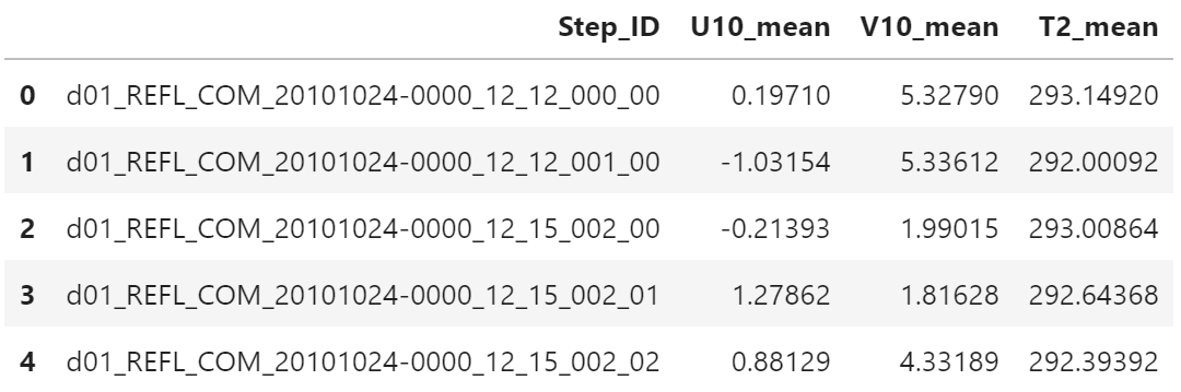
首先，让我们使用 key 列表找到的标签，将数据的子集放入 DataFrame 对象中。

df1 = df.loc[:, ["Step_ID", "U10_mean", "V10_mean", "T2_mean"]]
df1.head()

一旦数据被放入到 DataFrame 中，可以使用下面的命令获得均值

df1["T2_mean"].mean()

289.4654436647762

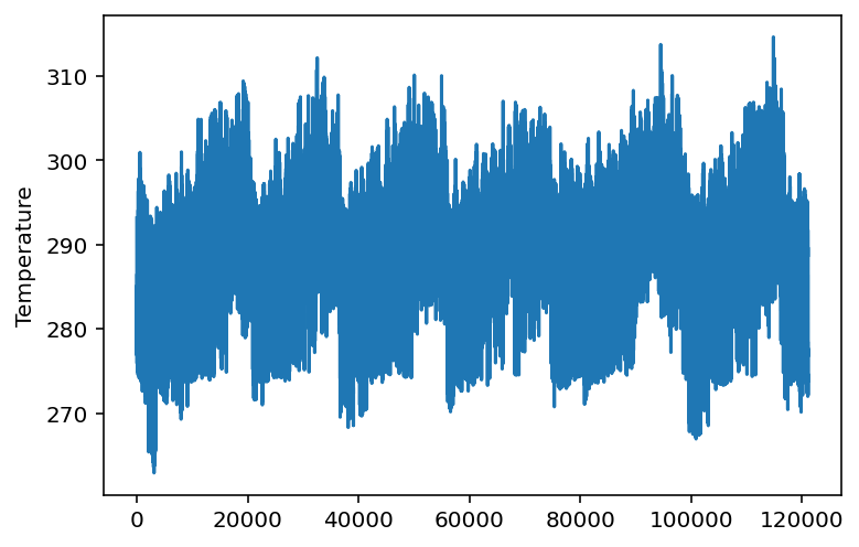
可以很容易创建快速图形

df1["T2_mean"].plot()
plt.ylabel("Temperature");

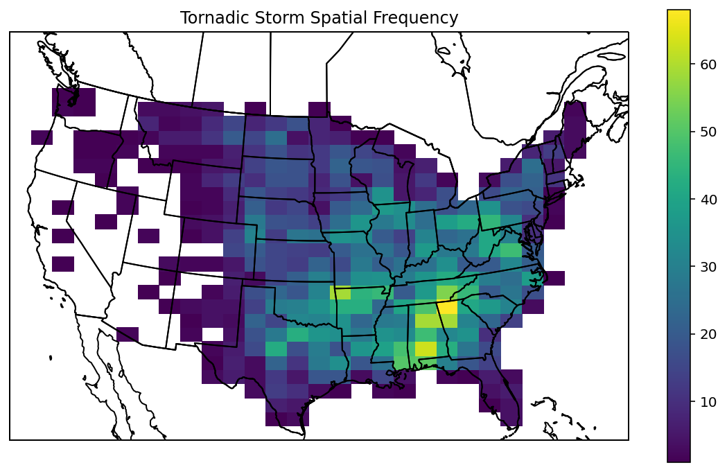
绘制复杂的图形

proj = ccrs.LambertConformal()
tor_index = df["RVORT1_MAX-future_max"] > 0.005
out_points = proj.transform_points(
    ccrs.PlateCarree(),
    df.loc[tor_index, "Centroid_Lon"].values,
    df.loc[tor_index, "Centroid_Lat"].values,
)

注：df.loc[var1, var2] 同时选择行和列的数据。

本例中，tor_index 表示行索引，并选择单个列 "Ceontroid_Lon"

df.loc[tor_index, "Centroid_Lon"].head()

335   -90.24486
336   -89.93511
338   -89.95105
339   -89.67590
340   -89.17130
Name: Centroid_Lon, dtype: float64

f.loc[tor_index, "Centroid_Lat"].head()

335    30.09427
336    30.12084
338    30.30276
339    30.45047
340    30.60191
Name: Centroid_Lat, dtype: float64

注：原始数据为等经纬度投影，即 ccrs.PlateCarree()，而绘制的地图使用兰勃脱投影，即 ccrs.LambertConformal()。所以使用 transform_points 函数，将数据的原始经纬度坐标转为兰勃脱投影对应的坐标。

out_points[:5]

array([[ 557928.35264405, -968829.10309901,       0.        ],
       [ 587715.73821425, -963918.79962841,       0.        ],
       [ 584823.82259096, -943777.38552494,       0.        ],
       [ 610238.74311549, -925538.86172077,       0.        ],
       [ 657574.3611661 , -905185.6773371 ,       0.        ]])

fig = plt.figure(
    figsize=(10, 6)
)
ax = fig.add_subplot(
    1, 1, 1,
    projection=proj
)

countries = cfeature.NaturalEarthFeature(
    "cultural", 
    "admin_0_countries", 
    "50m", 
    facecolor="None", 
    edgecolor="k"
)

states = cfeature.NaturalEarthFeature(
    "cultural", 
    "admin_1_states_provinces", 
    "50m", 
    facecolor="None", 
    edgecolor="k"
)

ax.add_feature(countries)
ax.add_feature(states)

out = ax.hist2d(
    out_points[:, 0],
    out_points[:, 1],
    bins=(
        np.linspace(-2.5e6, 2.5e6, 30),
        np.linspace(-1.5e6, 1.8e6, 30),
    ),
    cmin=1,
)

ax.set_extent(
    [-2.5e6, 2.5e6, -1.5e6, 1.8e6],
    crs=proj
)
plt.colorbar(out[-1])
plt.title("Tornadic Storm Spatial Frequency");

探索 NetCDF 文件

查找 NetCDF 文件

如果查找 NetCDF 文件并为找到的文件创建排序列表

为此，我们使用 pathlib 库列出指定目录中的所有 *.nc 文件。

# 创建 `pathlib.Path` 对象
path = pathlib.Path("../data/track_data_ncar_ams_3km_nc_small/")

# 查找 `path` 目录下的所有 nc 文件
files = sorted(path.glob("*.nc"))
files[:5]

[WindowsPath('../data/track_data_ncar_ams_3km_nc_small/NCARSTORM_20101024-0000_d01_model_patches.nc'),
 WindowsPath('../data/track_data_ncar_ams_3km_nc_small/NCARSTORM_20101122-0000_d01_model_patches.nc'),
 WindowsPath('../data/track_data_ncar_ams_3km_nc_small/NCARSTORM_20110201-0000_d01_model_patches.nc'),
 WindowsPath('../data/track_data_ncar_ams_3km_nc_small/NCARSTORM_20110308-0000_d01_model_patches.nc'),
 WindowsPath('../data/track_data_ncar_ams_3km_nc_small/NCARSTORM_20110326-0000_d01_model_patches.nc')]

读取第一个文件

读取第一个文件，并查看文件内容。

下面的代码中，我们打开文件列表中的第一个文件，并打印摘要信息。然后，我们关闭文件。

# 使用 NetCDF 库打开文件读取内容，然后关闭
nf = nc.Dataset(files[0], "r")
print(nf)
nf.close()

<class 'netCDF4._netCDF4.Dataset'>
root group (NETCDF4 data model, file format HDF5):
    Conventions: CF-1.6
    title: NCARSTORM Storm Patches for run 20101024-0000 member d01
    object_variable: REFL_COM
    dimensions(sizes): p(1472), row(32), col(32)
    variables(dimensions): int32 p(p), int32 row(row), int32 col(col), float32 lon(p,row,col), float32 lat(p,row,col), int32 i(p,row,col), int32 j(p,row,col), float32 x(p,row,col), float32 y(p,row,col), int32 masks(p,row,col), int32 time(p), float32 centroid_lon(p), float32 centroid_lat(p), float32 centroid_i(p), float32 centroid_j(p), int32 track_id(p), int32 track_step(p), float32 REFL_COM_curr(p,row,col), float32 U10_curr(p,row,col), float32 V10_curr(p,row,col), float32 T2_curr(p,row,col), float32 RVORT1_MAX_future(p,row,col), float32 HAIL_MAXK1_future(p,row,col)
    groups:

使用 xarray 打开文件

下面使用 xarray 打开文件，并输出内容。可以看到，输出的格式更易读。

xf = xr.open_dataset(files[0])
xf

<xarray.Dataset>
Dimensions:            (col: 32, p: 1472, row: 32)
Coordinates:
  * p                  (p) int32 0 1 2 3 4 5 6 ... 1466 1467 1468 1469 1470 1471
  * row                (row) int32 0 1 2 3 4 5 6 7 8 ... 24 25 26 27 28 29 30 31
  * col                (col) int32 0 1 2 3 4 5 6 7 8 ... 24 25 26 27 28 29 30 31
Data variables:
    lon                (p, row, col) float32 ...
    lat                (p, row, col) float32 ...
    i                  (p, row, col) int32 ...
    j                  (p, row, col) int32 ...
    x                  (p, row, col) float32 ...
    y                  (p, row, col) float32 ...
    masks              (p, row, col) int32 ...
    time               (p) datetime64[ns] ...
    centroid_lon       (p) float32 ...
    centroid_lat       (p) float32 ...
    centroid_i         (p) float32 ...
    centroid_j         (p) float32 ...
    track_id           (p) int32 ...
    track_step         (p) int32 ...
    REFL_COM_curr      (p, row, col) float32 ...
    U10_curr           (p, row, col) float32 ...
    V10_curr           (p, row, col) float32 ...
    T2_curr            (p, row, col) float32 ...
    RVORT1_MAX_future  (p, row, col) float32 ...
    HAIL_MAXK1_future  (p, row, col) float32 ...
Attributes:
    Conventions:      CF-1.6
    title:            NCARSTORM Storm Patches for run 20101024-0000 member d01
    object_variable:  REFL_COM

查看数据的不同部分

xarray 中有多种方法查看 NetCDF 文件的不同部分。

您可以在 xarray 对象中将键值引用变量。

可以使用变量的属性引用维度、表表和变量的属性。

T = xf["T2_curr"]
T

<xarray.DataArray 'T2_curr' (p: 1472, row: 32, col: 32)>
[1507328 values with dtype=float32]
Coordinates:
  * p        (p) int32 0 1 2 3 4 5 6 7 ... 1465 1466 1467 1468 1469 1470 1471
  * row      (row) int32 0 1 2 3 4 5 6 7 8 9 ... 22 23 24 25 26 27 28 29 30 31
  * col      (col) int32 0 1 2 3 4 5 6 7 8 9 ... 22 23 24 25 26 27 28 29 30 31
Attributes:
    long_name:  T2
    units:

维度

T.dims

('p', 'row', 'col')

坐标

T.coords

Coordinates:
  * p        (p) int32 0 1 2 3 4 5 6 7 ... 1465 1466 1467 1468 1469 1470 1471
  * row      (row) int32 0 1 2 3 4 5 6 7 8 9 ... 22 23 24 25 26 27 28 29 30 31
  * col      (col) int32 0 1 2 3 4 5 6 7 8 9 ... 22 23 24 25 26 27 28 29 30 31

属性

T.attrs

{'long_name': 'T2', 'units': ''}

索引和选择数据范围

有多种方法从变量中检索数值。

可以使用类似 numpy 数组的方法进行索引。也可以使用维度名称。

T[0, 0, 1]

<xarray.DataArray 'T2_curr' ()>
array(293.50546, dtype=float32)
Coordinates:
    p        int32 0
    row      int32 0
    col      int32 1
Attributes:
    long_name:  T2
    units:

T[0:5, 0, 1]

<xarray.DataArray 'T2_curr' (p: 5)>
array([293.50546, 293.06808, 294.17676, 294.1718 , 292.86124], dtype=float32)
Coordinates:
  * p        (p) int32 0 1 2 3 4
    row      int32 0
    col      int32 1
Attributes:
    long_name:  T2
    units:

T.sel(p=slice(0, 5), col=1, row=1)

<xarray.DataArray 'T2_curr' (p: 6)>
array([293.6699 , 293.06543, 294.07272, 293.9805 , 293.1326 , 293.39987],
      dtype=float32)
Coordinates:
  * p        (p) int32 0 1 2 3 4 5
    row      int32 1
    col      int32 1
Attributes:
    long_name:  T2
    units:

T.sel(p=4, col=1, row=0)

<xarray.DataArray 'T2_curr' ()>
array(292.86124, dtype=float32)
Coordinates:
    p        int32 4
    row      int32 0
    col      int32 1
Attributes:
    long_name:  T2
    units:

T.sel(row=0, col=1, p=4)

<xarray.DataArray 'T2_curr' ()>
array(292.86124, dtype=float32)
Coordinates:
    p        int32 4
    row      int32 0
    col      int32 1
Attributes:
    long_name:  T2
    units:

数据变换

下面的示例中，我们将使用 xarray 对象。

创建值大于 290 的数组，并将小于等于 290 的值设置为 nan。

T.where(T>290)

<xarray.DataArray 'T2_curr' (p: 1472, row: 32, col: 32)>
array([[[293.5103 , 293.50546, 292.88248, ..., 292.40265, 292.29697,
         292.0353 ],
       ...,
        [      nan,       nan,       nan, ...,       nan,       nan,
               nan]]], dtype=float32)
Coordinates:
  * p        (p) int32 0 1 2 3 4 5 6 7 ... 1465 1466 1467 1468 1469 1470 1471
  * row      (row) int32 0 1 2 3 4 5 6 7 8 9 ... 22 23 24 25 26 27 28 29 30 31
  * col      (col) int32 0 1 2 3 4 5 6 7 8 9 ... 22 23 24 25 26 27 28 29 30 31
Attributes:
    long_name:  T2
    units:

创建一个数据，大于 290 的值设为 True，小于等于 290 的值设为 False

T > 290

<xarray.DataArray 'T2_curr' (p: 1472, row: 32, col: 32)>
array([[[ True,  True,  True, ...,  True,  True,  True],
        ...,
        [False, False, False, ..., False, False, False]]])
Coordinates:
  * p        (p) int32 0 1 2 3 4 5 6 7 ... 1465 1466 1467 1468 1469 1470 1471
  * row      (row) int32 0 1 2 3 4 5 6 7 8 9 ... 22 23 24 25 26 27 28 29 30 31
  * col      (col) int32 0 1 2 3 4 5 6 7 8 9 ... 22 23 24 25 26 27 28 29 30 31

将所有值舍入到最接近的整数

T.round(0)

<xarray.DataArray 'T2_curr' (p: 1472, row: 32, col: 32)>
array([[[294., 294., 293., ..., 292., 292., 292.],
        [294., 294., 294., ..., 292., 292., 292.],
        [294., 294., 294., ..., 292., 292., 292.],
        ...,
        [283., 283., 283., ..., 276., 277., 276.],
        [283., 283., 284., ..., 277., 279., 279.],
        [283., 284., 285., ..., 279., 281., 281.]]], dtype=float32)
Coordinates:
  * p        (p) int32 0 1 2 3 4 5 6 7 ... 1465 1466 1467 1468 1469 1470 1471
  * row      (row) int32 0 1 2 3 4 5 6 7 8 9 ... 22 23 24 25 26 27 28 29 30 31
  * col      (col) int32 0 1 2 3 4 5 6 7 8 9 ... 22 23 24 25 26 27 28 29 30 31

查找该变量的所有值的平均值

T.mean()

<xarray.DataArray 'T2_curr' ()>
array(285.3192, dtype=float32)

T.mean(dim=["col", "row", "p"])

<xarray.DataArray 'T2_curr' ()>
array(285.3192, dtype=float32)

T.mean(dim=["col", "row"])

<xarray.DataArray 'T2_curr' (p: 1472)>
array([293.16837, 292.16022, 292.98077, ..., 281.79953, 282.82028,
       278.3346 ], dtype=float32)
Coordinates:
  * p        (p) int32 0 1 2 3 4 5 6 7 ... 1465 1466 1467 1468 1469 1470 1471

寻找变量所有值的最小值

T.max()

<xarray.DataArray 'T2_curr' ()>
array(303.61737, dtype=float32)

沿行列寻找最大值

T.max(dim=["col", "row"])

<xarray.DataArray 'T2_curr' (p: 1472)>
array([296.53342, 295.33218, 295.74823, ..., 284.14084, 286.5378 ,
       285.0278 ], dtype=float32)
Coordinates:
  * p        (p) int32 0 1 2 3 4 5 6 7 ... 1465 1466 1467 1468 1469 1470 1471

计算沿 p 轴第 5 百分位数的值

T.groupby('p').reduce(np.percentile, dim=('col', 'row'), q=5)

<xarray.DataArray 'T2_curr' (p: 1472)>
array([291.84577942, 291.11324921, 292.00157623, ..., 279.55417938,
       280.14920044, 272.69162445])
Coordinates:
  * p        (p) int32 0 1 2 3 4 5 6 7 ... 1465 1466 1467 1468 1469 1470 1471

使用 matplotlib 探索可视化

与使用 Python 所做的任何事情一样，有多种方法可以完成同一件事。以下是创建图的几种方法。

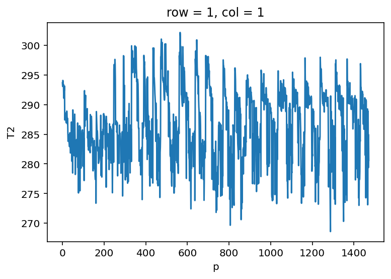
创建最简单的图形

T[:, 1, 1].plot();

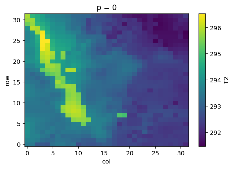
为 p=0 创建简单图形

T.isel(p=0).plot();

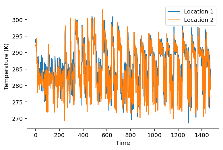
使用 Matplotlib 为两个地点创建时间序列图

注：p 代表时间，row 和 col 代表位置

plt.plot(
    xf["p"], 
    T[:, 1, 1], 
    label="Location 1",
)
plt.plot(
    xf["p"],
    T[:, 30, 30],
    label="Location 2",
)
plt.ylabel("Temperature (K)")
plt.xlabel("Time")
plt.legend();

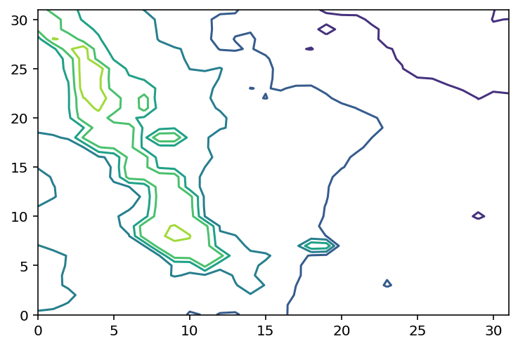
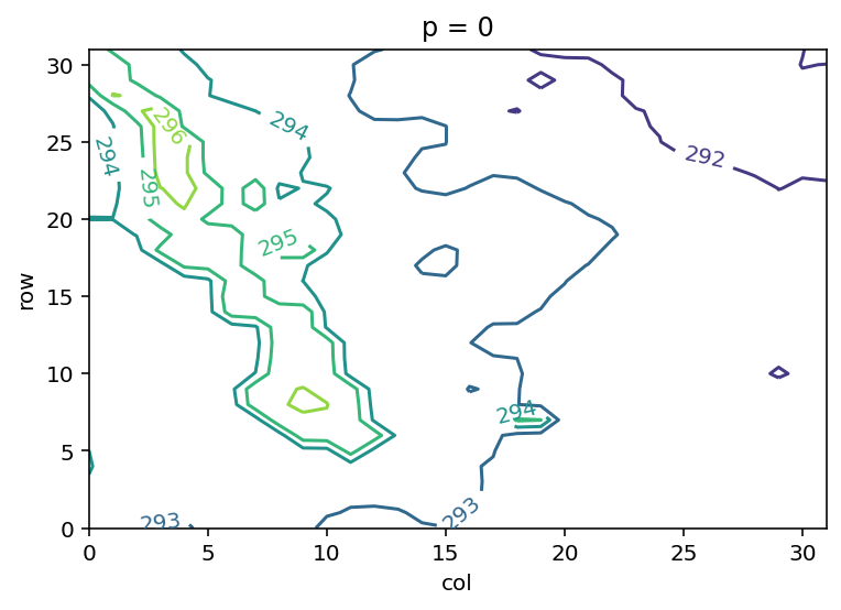
使用 Matploblib 创建简单等值线图

plt.contour(T[0, :, :]);

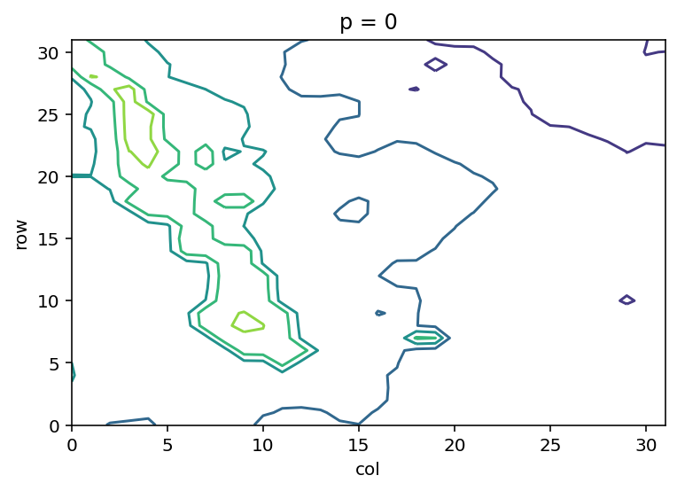
绘制与上图一样的图形，但使用 xarray 提供的坐标轴标签

T.sel(p=0).plot.contour();

和上面相同，但添加了等值线标签

cs = T.sel(p=0).plot.contour()
plt.clabel(
    cs, 
    fmt='%.0f', 
    inline=True
);

设置下面示例中使用的一些变量

V = xf["V10_curr"]
U = xf["U10_curr"]
r = xf["row"]
c = xf["col"]

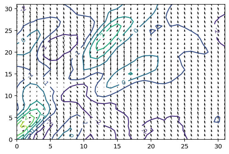
绘制等值线 + 风场箭头

cs = plt.contour(U.sel(p=0))
plt.clabel(
    cs,
    fmt="%.0f",
    inline=True,
)
plt.quiver(
    r, c, U.sel(p=0), V.sel(p=0),
    pivot="middle",
);

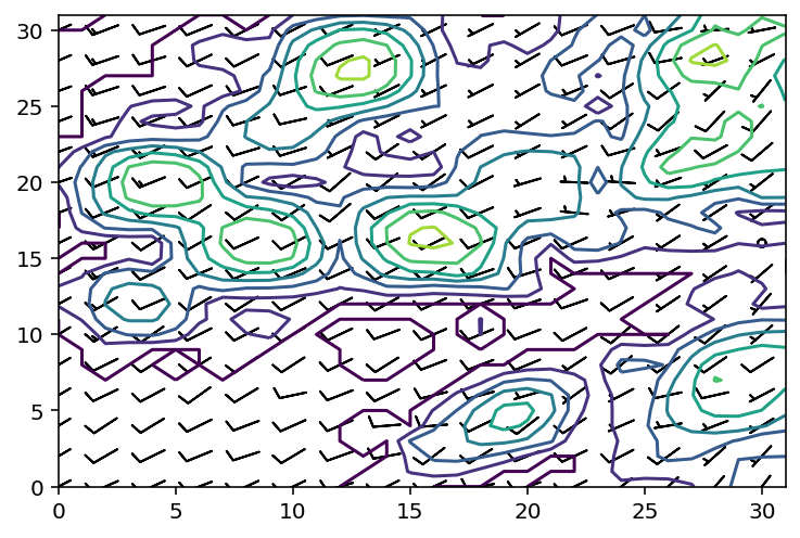
绘制风羽图

stride = 2
patch = 322
plt.contour(
    xf["REFL_COM_curr"].sel(p=patch)
)
plt.barbs(
    r[::stride], c[::stride],
    U.sel(p=patch)[::stride, ::stride],
    V.sel(p=patch)[::stride, ::stride],
    length=5,
    pivot="middle",
);

为教程准备数据

声明所有的输入和输出变量

run_times = []
valid_times = []

in_vars = [
    "REFL_COM_curr",
    "U10_curr",
    "V10_curr",
]

out_vars = ["RVORT1_MAX_future"]

in_data = []
out_data = []

遍历所有文件，提取相关的变量

for f in files:
    run_time = pd.Timestamp(f.name.split("_")[1])
    ds = xr.open_dataset(f)
    in_data.append(
        np.stack([
            ds[v].values for v in in_vars
        ], axis=-1)
    )
    out_data.append(
        np.stack([
            ds[v].values for v in out_vars
        ], axis=-1)
    )
    valid_times.append(ds["time"].values)
    run_times.append([run_time] * in_data[-1].shape[0])
    ds.close()

单个输入数据：时间 -> 行 -> 列 -> 变量

列表：不同文件

in_data[0].shape

(1472, 32, 32, 3)

将数据堆叠到单个数组中，而不是数组列表

这样做是为了更轻松地将数据馈送到机器学习算法中

文件 x 时间 -> 行 -> 列 -> 变量

all_in_data = np.vstack(in_data)
all_out_data = np.vstack(out_data)
all_in_data.shape

(121137, 32, 32, 3)

一维数组：文件 x 时间

all_run_times = np.concatenate(run_times)
all_valid_times = np.concatenate(valid_times)
all_run_times.shape

(121137,)

释放临时数组列表以节省内存

del in_data[:], out_data[:], run_times[:], valid_times[:]
del in_data, out_data, run_times, valid_times

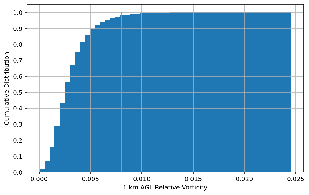
查找文件中的最大涡度值

注：每个时间点的最大涡度值

max_vorticity = all_out_data[:, :, :, 0].max(axis=-1).max(axis=-1)
vorticity_thresh = 0.008
percentileofscore(max_vorticity, vorticity_thresh)

97.47888754055326

根据阈值计算标签

vorticity_labels = np.where(max_vorticity > vorticity_thresh, 1, 0)
vorticity_labels

array([0, 0, 0, ..., 0, 0, 0])

创建直方图显示数据的分布

绘制输出变量的累计直方图

plt.figure(figsize=(8, 5))

# 绘制累计直方图
plt.hist(
    max_vorticity,
    bins=50,
    cumulative=True,
    density=True,
)

# 绘制阈值直线
plt.plot(
    np.ones(10) * vorticity_thresh, np.linspace(0, 1, 10)
)

plt.yticks(np.arange(0, 1.1, 0.1))
plt.grid()
plt.xlabel("1 km AGL Relative Vorticity")
plt.ylabel("Cumulative Distribution")

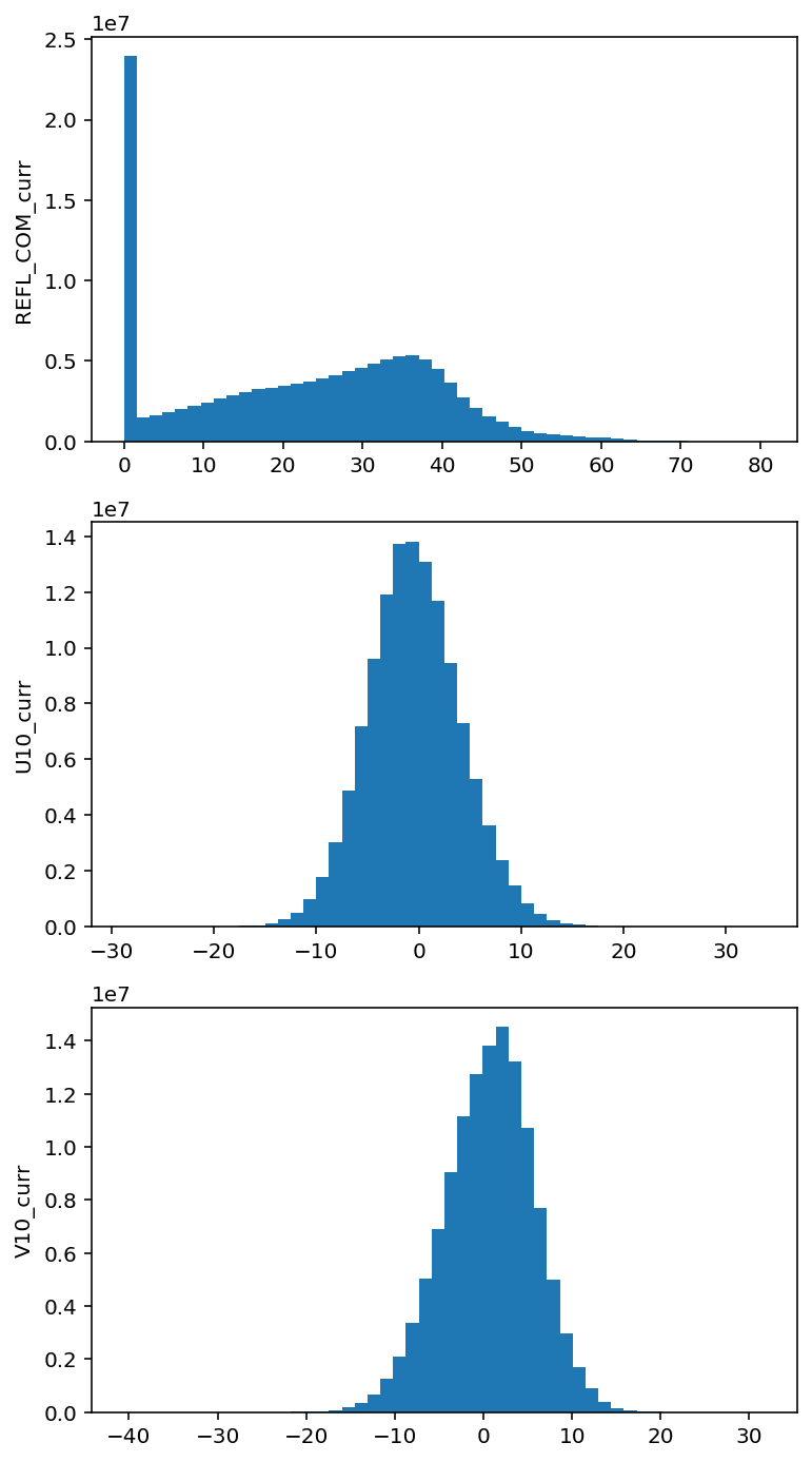
绘制输入变量的直方图

fig, axes = plt.subplots(
    all_in_data.shape[-1], 
    1,
    figsize=(6, all_in_data.shape[-1] * 4)
)
for a, ax in enumerate(axes):
    ax.hist(
        all_in_data[:, :, :, a].ravel(),
        50,
    )
    ax.set_ylabel(in_vars[a])

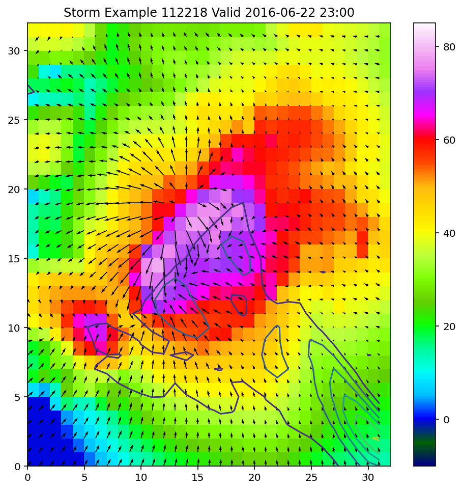
使用我们到目前为止所了解，绘制一个风暴示例

# 选择涡度值最大的风暴
rot_ex = max_vorticity.argmax()

plt.figure(figsize=(8, 8))

# 绘制反射率的彩色网格图
plt.pcolormesh(
    all_in_data[rot_ex, :, :, 0],
    cmap="gist_ncar",
    vmin=-10,
    vmax=85,
)
plt.colorbar()

# 绘制 U、V 风场箭头图
plt.quiver(
    all_in_data[rot_ex, :, :, 1],
    all_in_data[rot_ex, :, :, 2],
)

# 绘制涡度的等值线图
plt.contour(
    all_out_data[rot_ex, :, :, 0]
)

plt.title(
    f"Storm Example {rot_ex} "
    f"Valid {pd.Timestamp(all_valid_times[rot_ex]).strftime('%Y-%m-%d %H:%M')}"
);

分离训练集和测试集

我们需要将完整的数据集分成两个不同的组。第一组放入模型用于训练。第二组用于测试，查看模型是否按预期执行。通过了解数据来正确创建分组非常重要。例如，您的数据是否取决于时间？如果是这样，随机分配数据是否会使模型更难获取到数据模式？

选取要放入每个组中的正确数据量同样重要。选取不正确的数据量（以及选取不正确的组）可能会导致过拟合。当生成的模型进行预测时不够通用，将发生这种情况。

您可以尝试不同的组合，以查看它如何影响模型。

按日期

split_date = pd.Timestamp("2015-01-01")
train_indices = np.where(all_run_times < split_date)[0]
test_indices = np.where(all_run_times >= split_date)[0]
print(f"Size of training set: {len(train_indices)}")
print(f"Size of test set: {len(test_indices)}")

Size of training set: 76377
Size of test set: 44760

按随机索引

percent_train = .8

indices = np.arange(all_in_data.shape[0])
np.random.shuffle(indices)

split = int(indices.size * percent_train)
print("Splitting on index:", split)

train_indices = indices[:split]
test_indices = indices[split:]

print(f"Size of training set: {len(train_indices)}")
print(f"Size of test set: {len(test_indices)}")

Splitting on index: 96909
Size of training set: 96909
Size of test set: 24228

转换批量数据

一些机器学习模型对其输入变量的中心和方差敏感。默认情况下，神经网络会将其权重初始化为接近 0 的小值。因此，如果数据的均值不为 0 且标准差不为 1，则它们可能会难以收敛。通过重新缩放数据，我们可以帮助神经网络等模型更快收敛。一些预处理技术（例如 Prinicpal Component Analysis）也假设数据已标准化，并且如果违反该假设，将无法正常工作。

scikit-learn 为表格数据提供了多种缩放器。 StandardScaler 应用均值和标准差归一化，而 MinMaxScaler 重新缩放数据以适合固定范围。

from sklearn.preprocessing import MinMaxScaler, StandardScaler

refl = all_in_data[:, :, :, 0]

refl_stacked = refl.reshape(-1, refl.shape[1] * refl.shape[2])

scaler = StandardScaler()
scaler = scaler.fit(refl_stacked)
refl_norm = scaler.transform(refl_stacked)

refl_norm.shape

(121137, 1024)

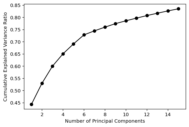
缩减维度

使用主成分分析（Principal Component Analysis(PCA)）对不同变量降维

主成分分析（PCA），也称为经验正交函数（以及其他名称的集合），是描述一组数据所需的降维技术。通过创建每个输入变量的加权加法组合，PCA 可用于减少数据的大小。主成分按它们解释数据的方差大小排序。最初生成主成分的奇异值分解与输入变量的数量具有相同的数量，但是以最小的方差量截断成分可以保留数据中最重要的部分，并删除其余部分。

要将 PCA 应用于空间数据，请先将每个图像展平为矢量，然后再应用 PCA。

from sklearn.decomposition import PCA

num_comps = 15
num_vars = refl_norm.shape[1]

pc_object = PCA(n_components=num_comps)
pc_train_data = pc_object.fit_transform(refl_norm[train_indices])
pc_test_data = pc_object.fit_transform(refl_norm[test_indices])

此图显示每个主成分的累积解释方差。

plt.plot(
    np.arange(1, num_comps + 1),
    np.cumsum(pc_object.explained_variance_ratio_),
    "ko-"
)
plt.xlabel("Number of Principal Components")
plt.ylabel("Cumulative Explained Variance Ratio")

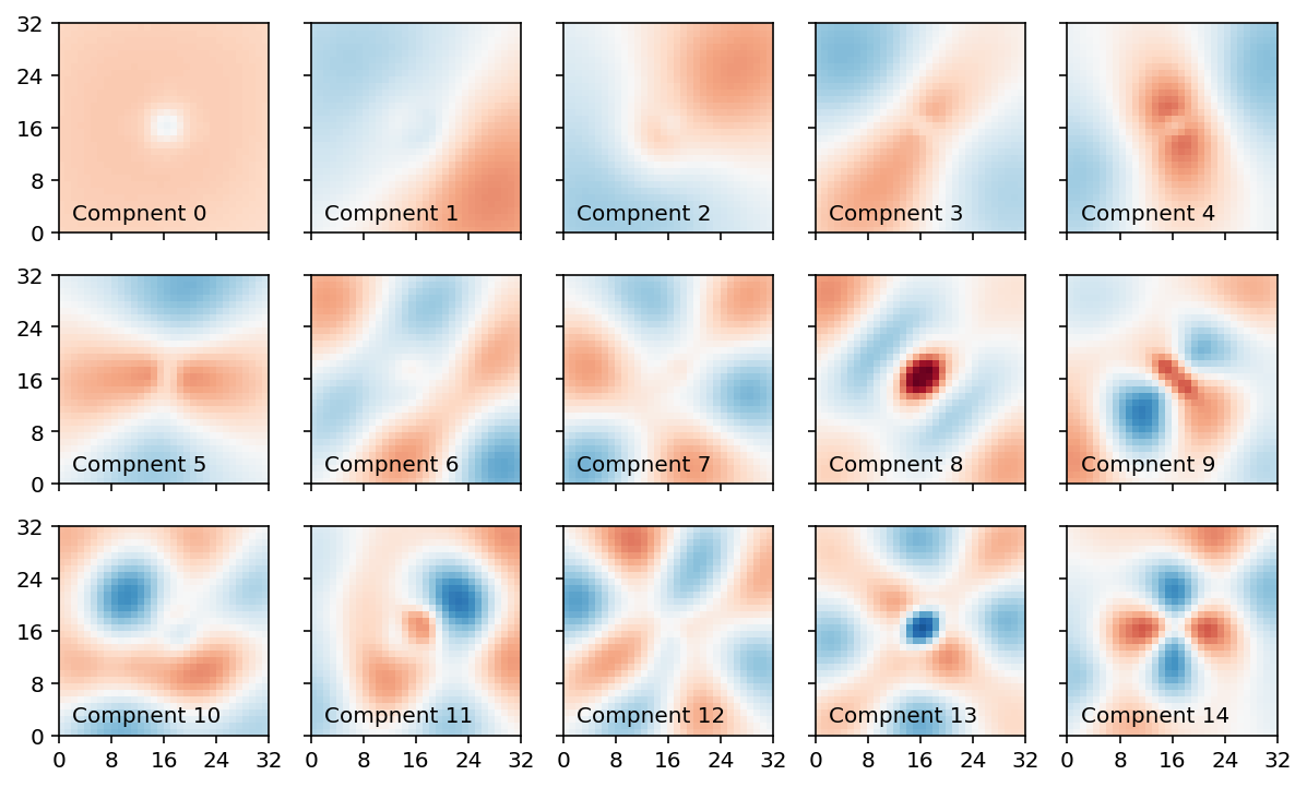
我们可以可视化每个组件的权重。权重的值受数据和域形状的影响。成分权重通常由随着成分数量的增加而增加频率的波浪模式组成。这些模式在许多数据集中都观察到，称为 Buell 模式。旋转 PCA 等方法可以降低 Buell 模式的影响，使权重更具可解释性，但代价是使权重不再正交。

fig, axes = plt.subplots(
    3, 5,
    figsize=(10, 6),
    sharex=True,
    sharey=True,
)
abs_max = np.max(np.abs(pc_object.components_))
for a, ax in enumerate(axes.ravel()):
    ax.pcolormesh(
        pc_object.components_[a].reshape(32, 32),
        vmin=-abs_max,
        vmax=abs_max,
        cmap="RdBu_r"
    )
    ax.text(
        2, 2,
        f"Compnent {a:d}",
    )
    ax.set_xticks(np.arange(0, 36, 8))
    ax.set_yticks(np.arange(0, 36, 8))

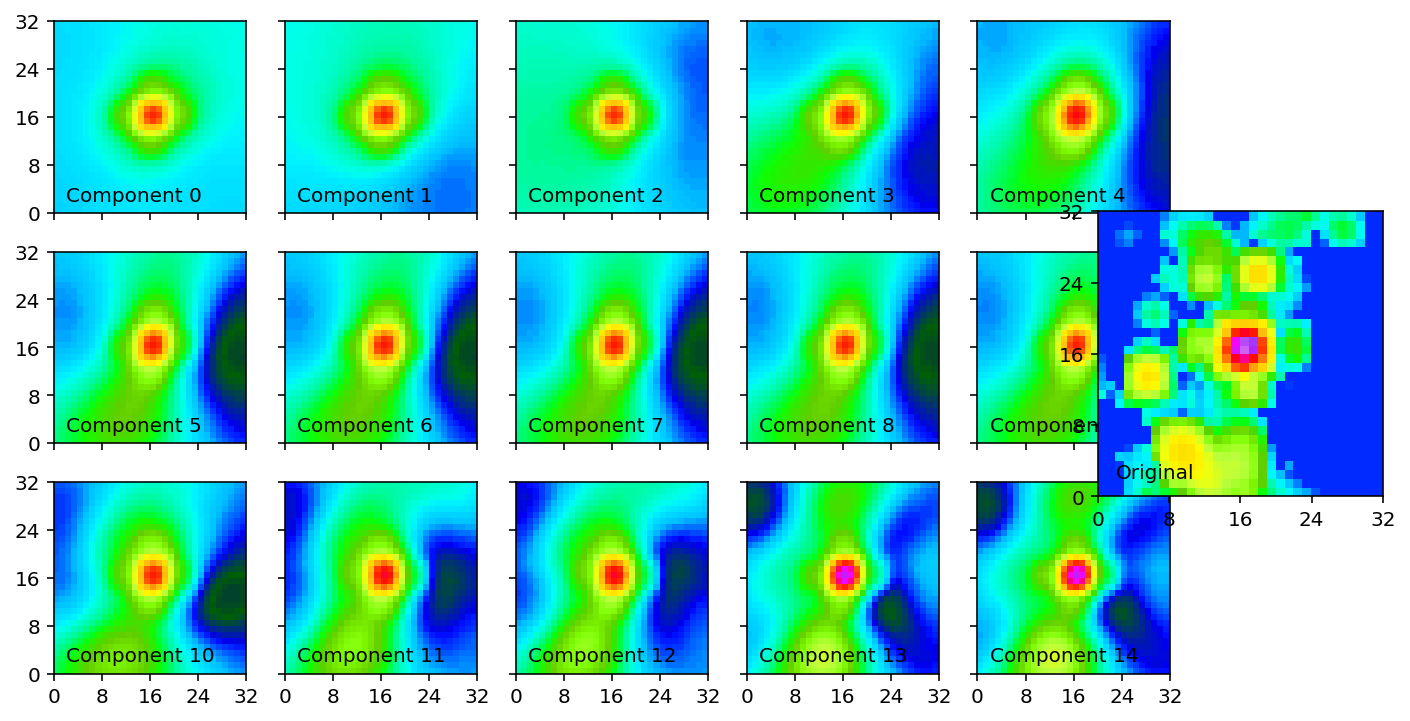
我们可以通过将更多主成分添加到一起来重建给定的示例。随着我们添加更多成分，更精细的缩放细节将重新出现。

pc_test_temp = np.zeros(
    pc_test_data.shape,
    dtype=np.float32,
)

fig, axes = plt.subplots(
    3, 5,
    figsize=(10, 6),
    sharex=True,
    sharey=True,
)
index = 1024

for a, ax in enumerate(axes.ravel()):
    pc_test_temp[:, a] = pc_test_data[:, a]
    inverse = scaler.inverse_transform(
        pc_object.inverse_transform(pc_test_temp)
    )
    ax.pcolormesh(
        inverse[index].reshape(32, 32),
        vmin=-10,
        vmax=75,
        cmap="gist_ncar",
    )
    ax.set_xticks(np.arange(0, 36, 8))
    ax.set_yticks(np.arange(0, 36, 8))
    ax.text(
        2, 2,
        f"Component {a:d}"
    )

ax_true = fig.add_axes([
    0.85, 0.33, 0.198, 0.33
])
ax_true.pcolormesh(
    all_in_data[test_indices][index][:, :, 0],
    vmin=-10,
    vmax=75,
    cmap="gist_ncar"
)
ax_true.set_xticks(np.arange(0, 36, 8))
ax_true.set_yticks(np.arange(0, 36, 8))
ax_true.text(2, 2, "Original");

all_out_data[test_indices][:, :, 0].max(axis=-1).max(axis=-1).argmax()

练习

将每个风暴的 V 风场转换为 10 个主成分。可视化成分权重，并查看每个成分为测试数据的示例风暴添加的特征。

参考

https://github.com/djgagne/ams-ml-python-course

AI4ESS 2020: 建立坚实的基础 - 定义机器学习问题和预处理