NWPC笔记:预测动态步长模式积分时长 - 线性回归
上一篇文章《NWPC笔记:分析动态步长模式积分时长 - 线性回归》中介绍如何使用线性回归拟合模式积分单步耗时,训练数据使用的是数据全集。
但在实时业务中,我们往往需要尽可能早地判断模式积分是否异常,也就需要在模式积分过程中使用已完成的积分步骤时间来预测积分结束时间。
本文介绍使用线性回归预测动态步长模式积分时长,对比使用不同的数据量作为训练集对最终预测结果的影响。 下面仅以 GRAPES MESO 3KM 模式系统为例进行说明。
声明:本文仅代表作者个人观点,所用数据无法代表真实情况,严禁转载。关于模式系统的相关信息,请以官方发布的信息及经过同行评议的论文为准。
获取数据
使用 nwpc-oper/nwpc-log-tool 工具获取积分单步耗时数据。
载入需要使用的库
import numpy as np
import pandas as pd
import matplotlib.pyplot as plt

from nwpc_log_tool.forecast_output.grapes_meso_3km import get_step_time_from_file
from nwpc_log_tool.data_finder import find_local_file
创建批量获取数据的函数
def get_cum_time(start_time_list):
    data = dict()
    for start_time in start_time_list:
        file_path = find_local_file(
            "grapes_meso_3km/log/fcst_ecf_out",
            start_time=start_time,
        )
        df = get_step_time_from_file(file_path)
        df["ctime"] = df["time"].cumsum()
        df["forecast_time"] = df["valid_time"] - start_time
        df["forecast_hour"] = (df["valid_time"] - start_time)/pd.Timedelta(hours=1)
        data[start_time] = df
    return data
获取 2020 年 4 月 10 日至 2020 年 4 月 30 日 00 时次的数据
data = get_cum_time(
    pd.date_range(
        "2020-04-10",
        "2020-04-30",
        freq="D"
    )
)
简单分析
计算积分总时间
final_time = [df["ctime"].iloc[-1]/60 for (key, df) in data.items()]
final_time = pd.Series(
    final_time,
    index=[key for key in data],
)
final_time
2020-04-10    58.076867
2020-04-11    57.163763
2020-04-12    56.837072
2020-04-13    92.715550
2020-04-14    58.393600
2020-04-15    56.972327
2020-04-16    57.076605
2020-04-17    75.252454
2020-04-18    59.959220
2020-04-19    61.972465
2020-04-20    63.409057
2020-04-21    61.339032
2020-04-22    59.573950
2020-04-23    56.343490
2020-04-24    57.780713
2020-04-25    58.387953
2020-04-26    55.689460
2020-04-27    56.633655
2020-04-28    56.942238
2020-04-29    94.794315
2020-04-30    58.870298
dtype: float64
绘制简单的线条图
final_time.plot()
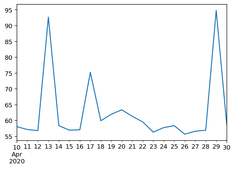
有三个时次的积分时长明显异常:
- 2020-04-13: 92 分钟
- 2020-04-17: 75 分钟
- 2020-04-29: 94 分钟
预测积分时长的目的就是尽可能早地发现这三个积分异常的时次,并且其他积分正常的时次不能被误判。
训练模型
使用 scikit-learn 的线性回归方法训练模型,训练数据从积分 3 小时以后的数据中选择。
因为上一篇文章中提到,3 小时的积分步骤耗时太长(超过 100 秒),对早期的预测结果影响太大。
创建训练单个模型的函数
from sklearn import linear_model

def get_linear_model(df, sample_hour):
    sample = df[df["forecast_hour"].between(3, sample_hour)]
    X = sample["forecast_hour"].values.reshape(-1, 1)
    y = sample["ctime"]
    reg = linear_model.LinearRegression()
    reg.fit(X, y)
    return reg
创建批量训练模型的函数
def get_linear_models(data, sample_hour):
    models = []
    for (key, df) in data.items():
        model = get_linear_model(df, sample_hour)
        models.append({
            "key": key,
            "model": model,
        })
    return models
从 6 小时开始,逐小时训练一个模型
hour_list = np.arange(6, 37, 1)
total_end_times = {}
total_coefs = {}
total_bias = {}
for hour in hour_list:
    models = get_linear_models(data, hour)
    end_times = []
    coefs = []
    for model in models:
        end_time = model["model"].predict(np.reshape(36, (-1, 1)))[0]/60
        end_times.append(end_time)
        coefs.append(model["model"].coef_[0])
    bias = end_times - final_time
    coefs = pd.Series(coefs, index=bias.index)
    total_end_times[hour] = end_times
    total_bias[hour] = bias
    total_coefs[hour] = coefs

end_times_df = pd.DataFrame(total_end_times, index=final_time.index)
bias_df = pd.DataFrame(total_bias)
coefs_df = pd.DataFrame(total_coefs)
分析
绘制线条图分析不同数据量对预测结果的影响。
积分时长
end_times_df 是预测的积分时长。
绘制多个模型的预测结果,并用红色表示实际积分时长。
fig, ax = plt.subplots(figsize=(15, 10))
ax.set_title("End time")
end_times_df.plot(
    cmap="viridis",
    ax=ax,
)
p = final_time.plot(
    color="red",
    ax=ax
)
p.legend(bbox_to_anchor=(1.1, 1.0))
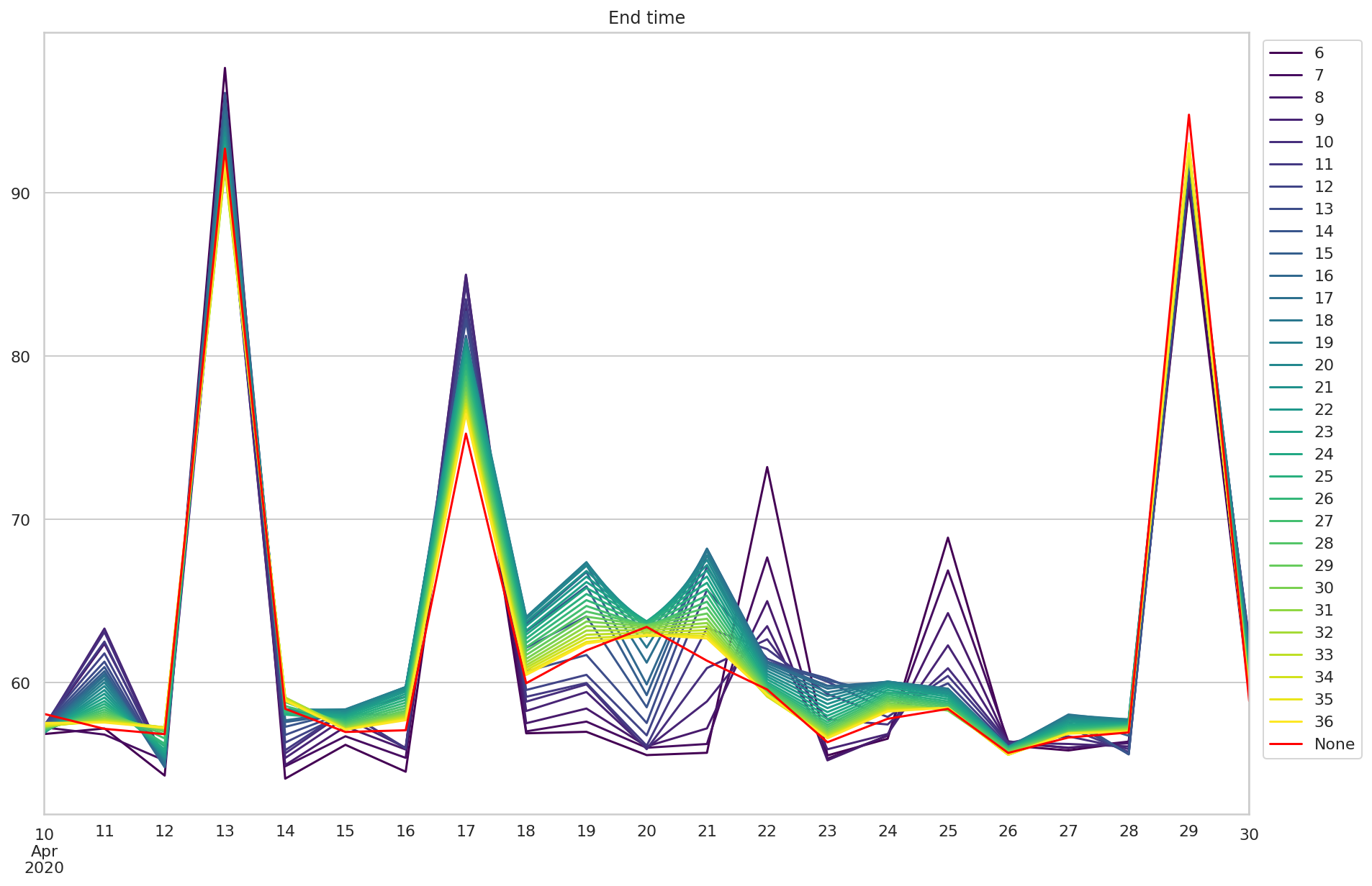
可以看到随着使用数据增多,预测结果越来越精确。 三个异常的时次也比较容易能分辨出。 但 4 月 22 日和 4 月 25 日的早期预测结果明显比实际结果偏大,会影响对积分是否异常的判断。
偏差
bias_df 是预测时长与实际时长的偏差。
fig, ax = plt.subplots(figsize=(15, 10))
ax.set_title("Bias")
p = bias_df.plot(
    cmap="viridis",
    ax=ax,
)
p.legend(bbox_to_anchor=(1.1, 1.0))
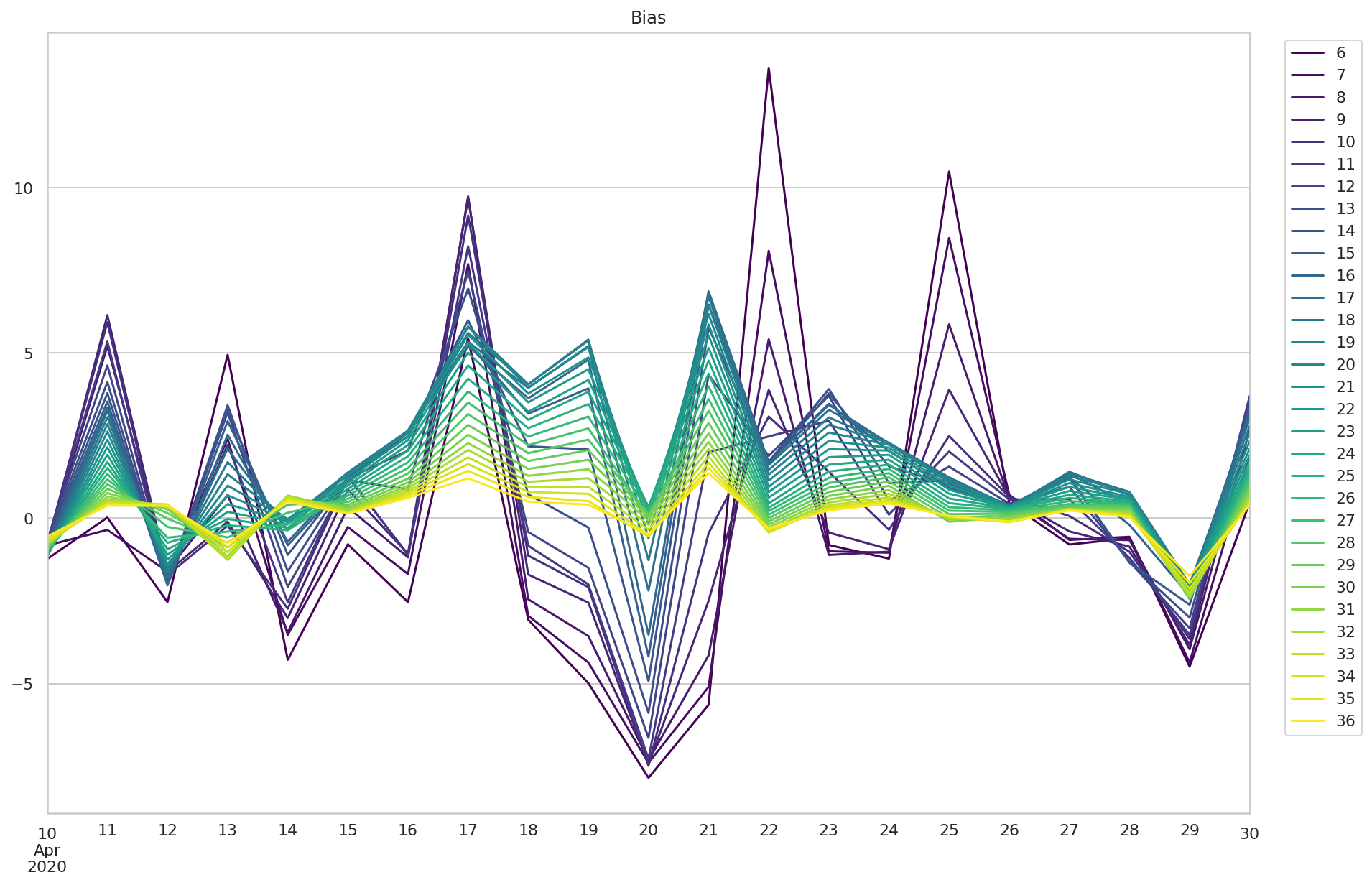
比较大的偏差来自 4 月 22 日和 25 日的早期预测,最大值在 12 分钟左右。
斜率
coef_df 是拟合直线的斜率
fig, ax = plt.subplots(figsize=(15, 10))
ax.set_title("Coef")
p = coefs_df.plot(
    cmap="viridis",
    ax=ax,
)
p.legend(bbox_to_anchor=(1.1, 1.0))
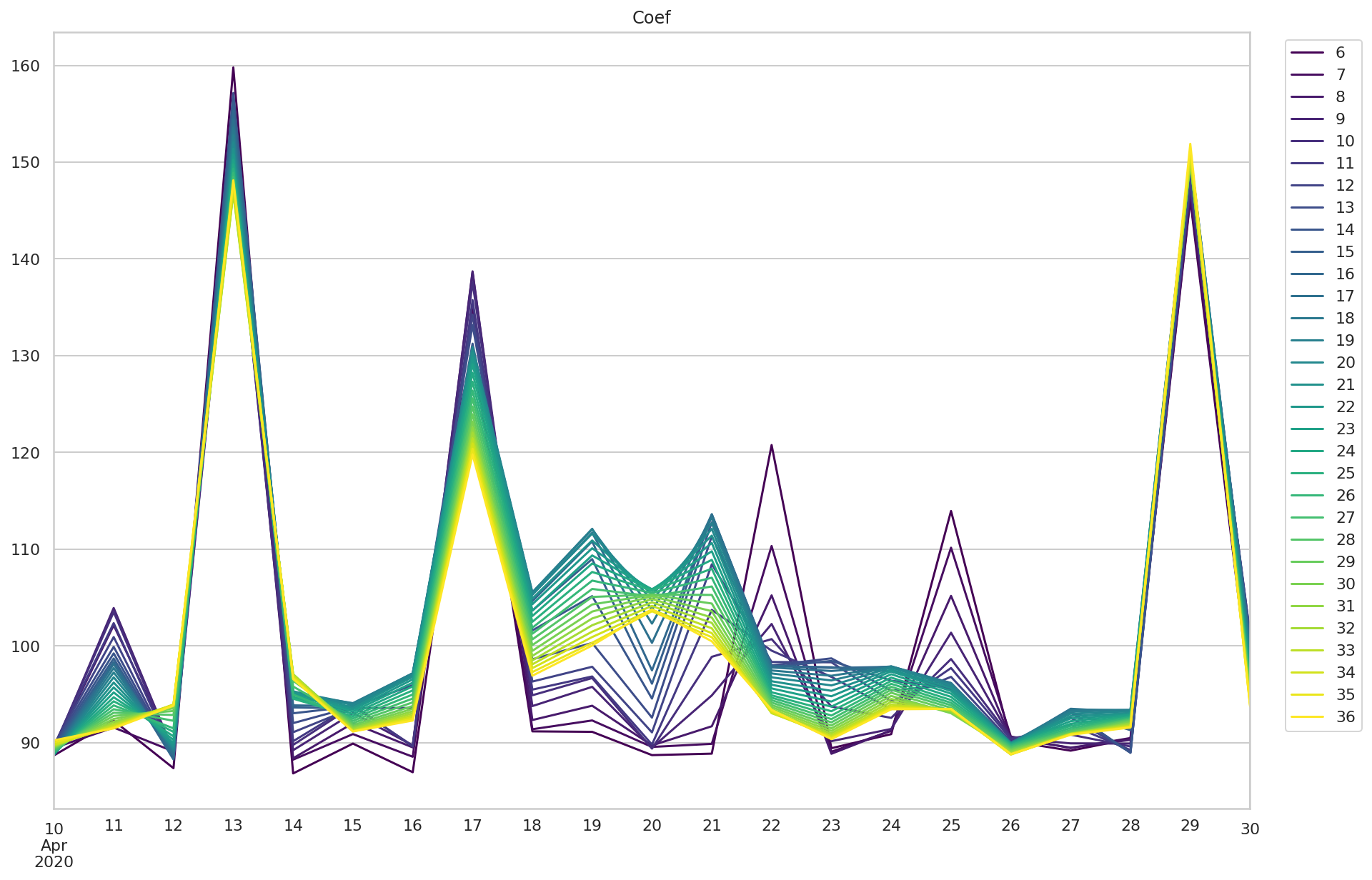
可以看到,积分异常的三个时次,拟合直线斜率在所有模型中都比较大。 但 4 月 22 日和 25 日的早期预测模型也展现了较大的斜率。
使用 seaborn 分析
线条图不容易看到变化趋势,下面绘制热度图进一步观察变化趋势。
积分时长
fig, ax = plt.subplots(figsize=(10, 5))
ax.set_title("End time")
end_times_plot_df = end_times_df.copy()
end_times_plot_df.index = end_times_plot_df.index.map(lambda x: x.strftime("%Y-%m-%d"))
ax = sns.heatmap(
    end_times_plot_df,
    cmap="YlOrRd",
    linewidths=.5,
    ax=ax,
)
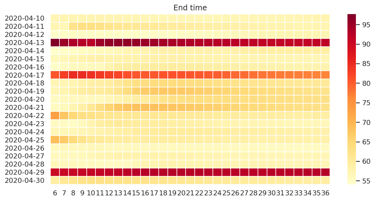
可以看到,积分异常的时次在所有训练模型中都有较大的积分时长。
对于 4 月 22 日和 25 日,虽然前几个模型预测结果有异常,但从 9 - 12 小时开始的后续结果基本保持一致。
偏差
使用蓝色表示偏差为负,使用红色表示偏差为正,使用白色表示没有偏差。
fig, ax = plt.subplots(figsize=(10, 5))
plot_df = bias_df.copy()
plot_df.index = plot_df.index.map(lambda x: x.strftime("%Y-%m-%d"))
ax.set_title("Bias")
ax = sns.heatmap(
    plot_df,
    cmap="seismic",
    center=0,
    linewidths=.5,
    ax=ax,
)
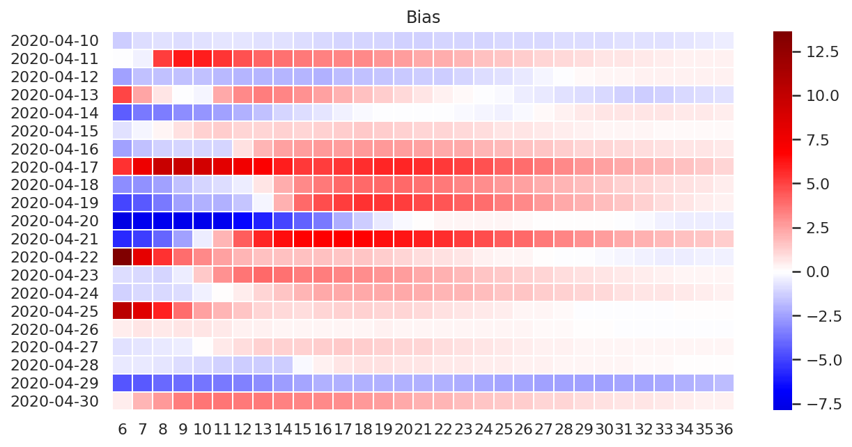
4 月 18 日,19 日和 21 日的变化比较特殊,中间时效训练的模型误差有一定程度的增大。
不同时次的误差变化模式不太一致,有待笔者进一步分析研究。
斜率
fig, ax = plt.subplots(figsize=(10, 5))
ax.set_title("Coef")
coefs_plot_df = coefs_df.copy()
coefs_plot_df.index = coefs_plot_df.index.map(lambda x: x.strftime("%Y-%m-%d"))
ax = sns.heatmap(
    coefs_plot_df,
    cmap="YlOrRd",
    linewidths=.5,
    ax=ax,
)
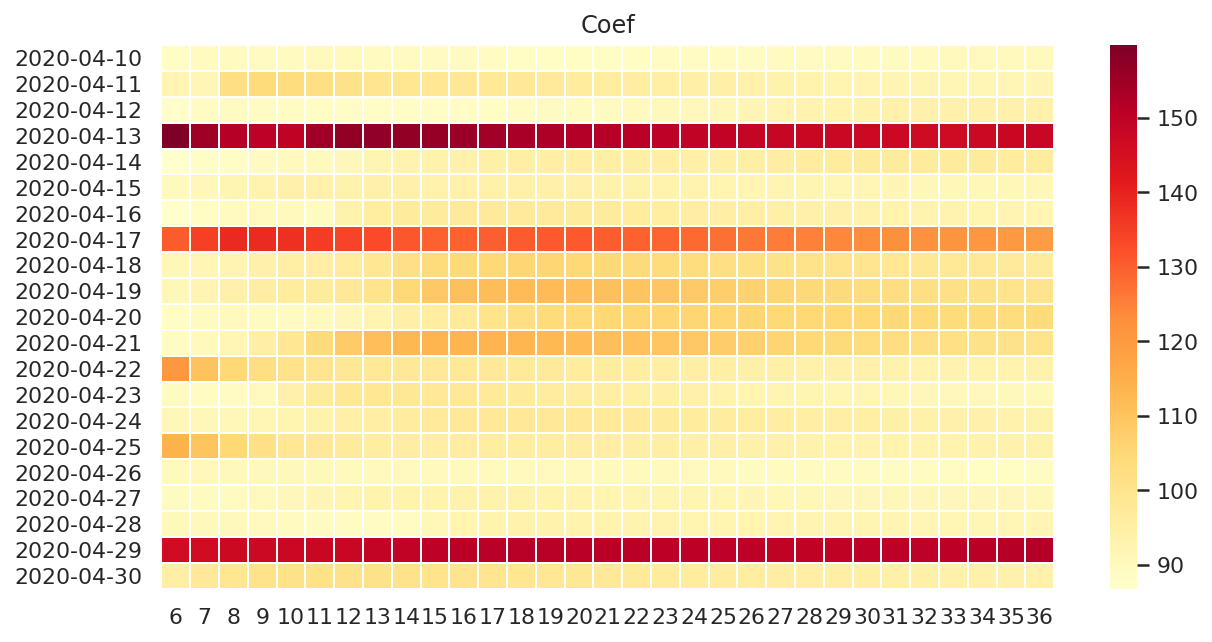
可以看到,积分异常的时次在所有训练模型中都有较大的斜率。
对于 4 月 22 日和 25 日,虽然前几个模型斜率较大,但从 9 - 12 小时开始的后续斜率基本保持一致。
与误差相似,4 月 18 日,19 日和 20 日的中间时效训练模型的斜率也有一定程度的增加,有待进一步研究。
总结
动态步长模式时长预测明显难于固定步长,但还是可以大体通过斜率判断积分是否异常。 不过需要注意,早期的预测结果不一定能反映实际的情况。
