NWPC笔记:分析动态步长模式积分时长 - 线性回归
之前的文章《NWPC笔记:对比模式积分时长 - 动态步长》中提到动态步长的模式积分单步耗时累计时间在正常情况和异常情况下也有不同的斜率。
本文介绍使用线性回归拟合动态步长模式积分单步耗时,并对比两种情况下线性拟合的效果。 下面以 GRAPES MESO 3KM 为例进行说明。
声明:本文仅代表作者个人观点,所用数据无法代表真实情况,严禁转载。关于模式系统的相关信息,请以官方发布的信息及经过同行评议的论文为准。
获取数据
使用《NWPC笔记:对比模式积分时长 - 动态步长》中提到的 2020 年 4 月 13 日(异常情况)和 2020 年 4 月 22 日(正常情况)两个数据。 具体获取方法请查看该文章,不再详细介绍。
下面首先以 2020 年 4 月 22 日的数据为例说明如何进行线性拟合。
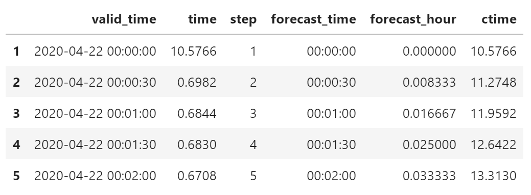
假设数据已被加载到 df 中,对数据进行一定的处理。
为了方便计算和显示,使用浮点类型的预报小时 forecat_hour 作为自变量。
df = get_step_time_from_file(file_path)
df["step"] = df.index
df["forecast_time"] = df["valid_time"] - start_time
df["forecast_hour"] = (df["valid_time"] - start_time)/pd.Timedelta(hours=1)
df["ctime"] = df["time"].cumsum()
df.head()
使用 Seaborn 绘制线性拟合曲线
Seaborn 内置了线性拟合功能。
import seaborn as sns
sns.set(style="whitegrid")
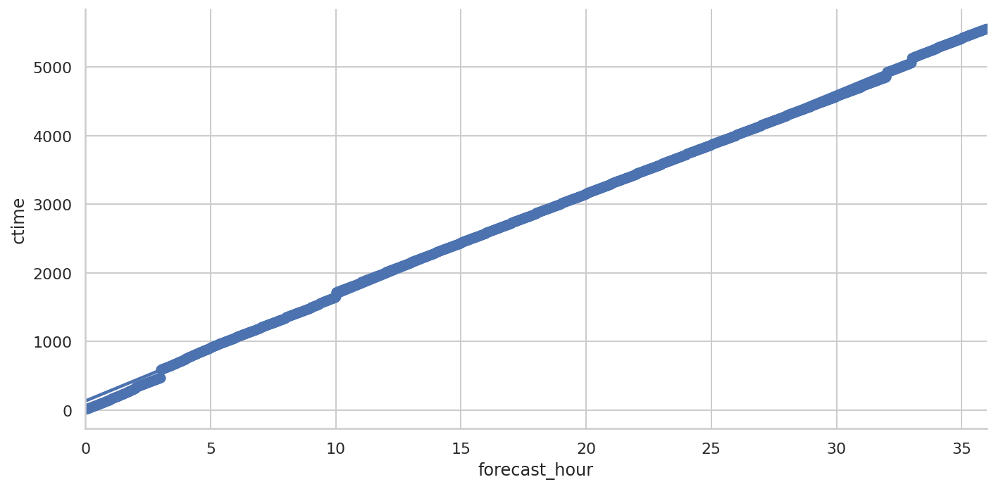
sns.lmplot(
x="forecast_hour",
y="ctime",
data=df,
height=5,
aspect=2,
)
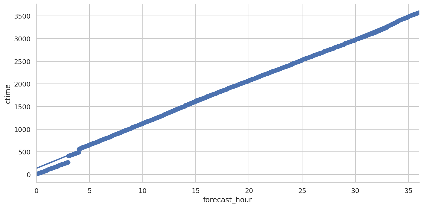
可以看到,3小时以内的数据拟合有明显的误差。 这是因为3小时的那一步需要运行很长时间(100秒左右),导致前后的累计时间有明显的跃升。
使用 scikit-learn 计算线性回归
使用 scikit-learn 提供的线性回归算法 LinearRegression 计算线性拟合。
from sklearn import linear_model
将积分步数处理成 scikit-learn 需要的二维变量。
X = df["forecast_hour"].values.reshape(-1, 1)
y = df["ctime"]
使用所有的数据训练线性回归模型(不是最好的方式)
model = linear_model.LinearRegression()
model.fit(X, y)
LinearRegression(copy_X=True, fit_intercept=True, n_jobs=None, normalize=False)
查看拟合直线的斜率和截距
model.coef_, model.intercept_
(array([95.6874529]), 136.96091594814493)
查看拟合的评分
model.score(X, y)
0.9976133038211057
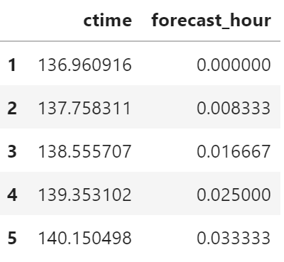
使用训练的模型计算累计时间
predict_df = pd.DataFrame(
    {
        "ctime": model.predict(
            df["forecast_hour"].values.reshape(-1, 1)
        ),
        "forecast_hour": df["forecast_hour"]
    },
    index=df.index
)
predict_df.head()
下面使用 Bokeh 绘制原始数据和预测数据的折线图。
from bokeh.io import output_notebook, show
from bokeh.plotting import figure
from bokeh.models import ColumnDataSource
output_notebook()
source = ColumnDataSource(df)
predict_source = ColumnDataSource(predict_df)
p = figure(
plot_height=500,
plot_width=1000,
title="MODEL B",
)
p.line(
x="forecast_hour",
y="ctime",
source=source,
color="red",
legend_label="real"
)
p.line(
x="forecast_hour",
y="ctime",
source=predict_source,
color="green",
legend_label="predict",
)
p.legend.location = "top_left"
p.xaxis.axis_label = "forecast hour"
p.yaxis.axis_label = "time(seconds)"
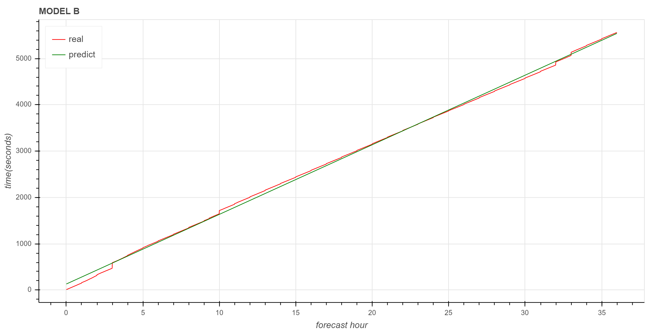
show(p)
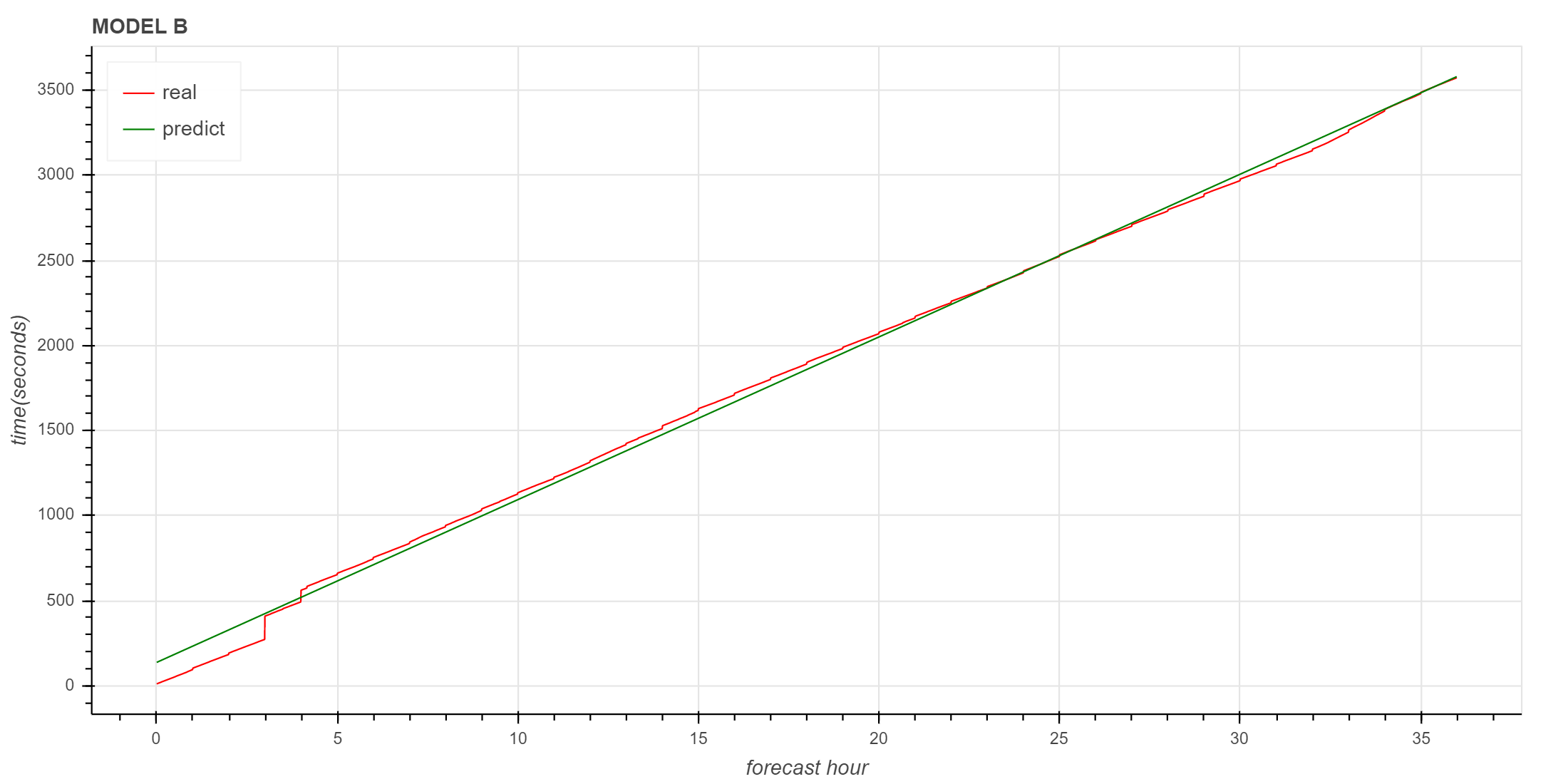
图中红色是实际曲线,绿色是拟合的直线,3小时以后的拟合直线很好地描述了实际数据的变化趋势。
异常情况
下面让我们再看一下异常情况下线性拟合的效果。
Seaborn
Seaborn 的线性拟合
拟合的曲线与实际数据基本一致。
Scikit-learn
使用 scikit-learn 训练线性回归模型
斜率和截距
(array([150.32393828]), 131.3590634848033)
拟合效果评分
0.9988721635715764
实际数据与拟合数据对比
同样可以看到,3小时以后的拟合直线与原始数据趋势基本一致。
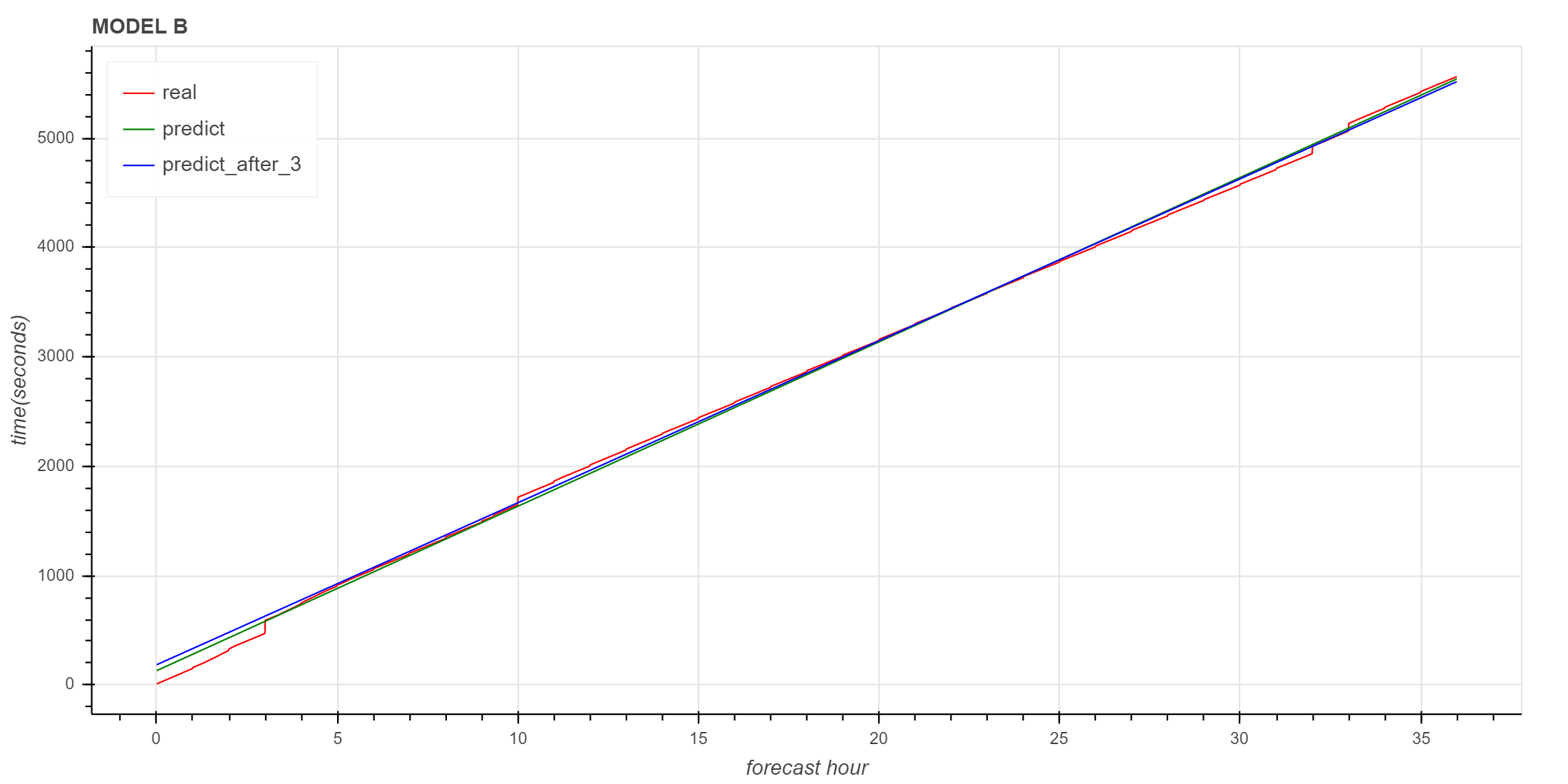
使用3小时以后的数据进行预测
下面是使用3小时以后的数据训练模型的对比,可以看到与使用全集数据基本一致。
进一步评估
下面查看 2020 年 4 月 10 日到 4 月 30 日的拟合结果。
获取数据
def get_cum_time(start_time_list):
    data = dict()
    for start_time in start_time_list:
        file_path = find_local_file(
            "grapes_meso_3km/log/fcst_ecf_out",
            start_time=start_time,
        )
        df = get_step_time_from_file(file_path)
        df["ctime"] = df["time"].cumsum()
        df["forecast_time"] = df["valid_time"] - start_time
        df["forecast_hour"] = (df["valid_time"] - start_time)/pd.Timedelta(hours=1)
        df["ctime"] = df["time"].cumsum()
        data[start_time] = df
    return data

data = get_cum_time(pd.date_range("2020-04-10", "2020-04-30", freq="D"))
显示总耗时
records = []
indexes = []
for (key, df) in data.items():
    record = {"total": df['ctime'].iloc[-1]/60}
    indexes.append(key)
    records.append(record)
total_df = pd.DataFrame(records, index=indexes)
total_df
2020-04-10	58.076867
2020-04-11	57.163763
2020-04-12	56.837072
2020-04-13	92.715550
2020-04-14	58.393600
2020-04-15	56.972327
2020-04-16	57.076605
2020-04-17	75.252454
2020-04-18	59.959220
2020-04-19	61.972465
2020-04-20	63.409057
2020-04-21	61.339032
2020-04-22	59.573950
2020-04-23	56.343490
2020-04-24	57.780713
2020-04-25	58.387953
2020-04-26	55.689460
2020-04-27	56.633655
2020-04-28	56.942238
2020-04-29	94.794315
2020-04-30	58.870298
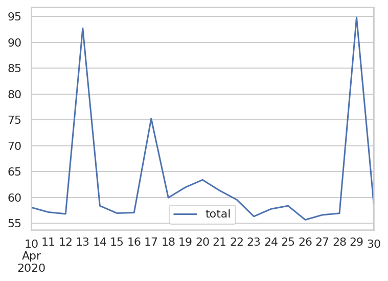
绘图展示总耗时变化
total_df.plot()
训练模型
创建训练模型的函数
def get_linear_models(data, days):
    models = []
    for key,df in data.items():
        X = df["forecast_hour"].values.reshape(-1, 1)
        y = df["ctime"]
        reg = linear_model.LinearRegression()
        reg.fit(X, y)
        models.append({
            "key": a,
            "model": reg,
        })
    return models
计算模型并输出拟合结果
predict_end_times = []
real_end_times = []
days = 10

for key,df in data.items():
    X = df["forecast_hour"].values.reshape(-1, 1)
    y = df["ctime"]
    reg = linear_model.LinearRegression()
    reg.fit(X, y)
    predict_end_time = reg.predict(np.reshape(36, (-1, 1)))[0]/60
    real_end_time = df["ctime"].iloc[-1]/60
    print(
        key,
        reg.coef_,
        real_end_time,
        predict_end_time,
    )
    real_end_times.append(real_end_time)
    predict_end_times.append(predict_end_time)
2020-04-10 00:00:00 [91.93795486] 58.0768666666668 57.84149304375201
2020-04-11 00:00:00 [93.4418504] 57.1637633333333 57.92636567977424
2020-04-12 00:00:00 [94.54772291] 56.83707166666681 57.353481623528516
2020-04-13 00:00:00 [150.32393828] 92.71554999999975 92.38368069050672
2020-04-14 00:00:00 [97.35188156] 58.39359999999969 59.042529299231575
2020-04-15 00:00:00 [92.89066492] 56.972326666666866 57.44825123770353
2020-04-16 00:00:00 [93.92975467] 57.07660500000009 58.01366398518585
2020-04-17 00:00:00 [123.14540758] 75.25245350000021 77.09141797823801
2020-04-18 00:00:00 [98.59538213] 59.95921999999995 60.789340280546334
2020-04-19 00:00:00 [101.76020314] 61.97246500000028 62.71095114372834
2020-04-20 00:00:00 [104.41972552] 63.40905666666672 63.04980146338114
2020-04-21 00:00:00 [102.26874771] 61.33903166666671 63.065273989889725
2020-04-22 00:00:00 [95.6874529] 59.57395000000001 59.69515367003884
2020-04-23 00:00:00 [92.02728587] 56.34349000000007 56.9061273968128
2020-04-24 00:00:00 [95.0309262] 57.78071316666673 58.53200075916805
2020-04-25 00:00:00 [95.25234337] 58.387953333333485 58.7954199798231
2020-04-26 00:00:00 [90.41329148] 55.689460000000096 55.88916380343838
2020-04-27 00:00:00 [92.54505008] 56.633655000000246 57.204836649660926
2020-04-28 00:00:00 [93.07738024] 56.9422383333333 57.26789479751935
2020-04-29 00:00:00 [153.25395767] 94.79431500000008 93.29470481559052
2020-04-30 00:00:00 [95.87403487] 58.87029833333306 59.68034665540815
上面输出中第二列是斜率,第三列是实际时间,第四列是拟合时间。 可以看到,积分耗时大的时次,拟合的斜率也比较大。
计算最后一步拟合结果与实际数据的偏差
pd.Series(predict_end_times) - pd.Series(real_end_times)
0    -0.235374
1     0.762602
2     0.516410
3    -0.331869
4     0.648929
5     0.475925
6     0.937059
7     1.838964
8     0.830120
9     0.738486
10   -0.359255
11    1.726242
12    0.121204
13    0.562637
14    0.751288
15    0.407467
16    0.199704
17    0.571182
18    0.325656
19   -1.499610
20    0.810048
dtype: float64
可以看到,误差都在 2 分钟以内。
使用全量数据训练模型没有太大意义,我们更关心是否能在模式运行阶段就预测出模式积分有异常,这就需要使用前面积分步骤的耗时数据来预测积分的总体趋势。 下一篇文章将尝试讨论使用部分数据预测的可行性。
