NWPC笔记：对比模式积分时长 - 动态步长

May 17, 2020 (最后修改: August 22, 2021)

上一篇文章《NWPC笔记：获取模式积分时长 - 动态步长》介绍如何获取动态步长的模式积分时长，并使用积分时间在正常范围内的时次（2020042200）作为示例。

本文进一步对比积分时间正常和异常的情况下积分时间的变化，同样只针对 GRAPES MESO 3KM 系统。

声明：本文仅代表作者个人观点，所用数据无法代表真实情况，严禁转载。关于模式系统的相关信息，请以官方发布的信息及经过同行评议的论文为准。

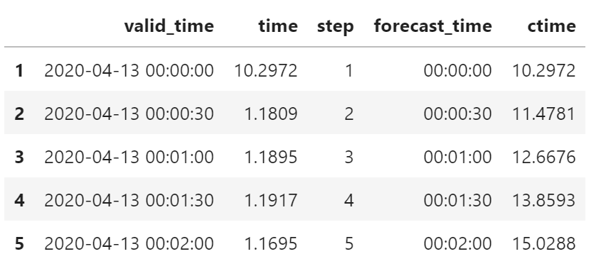
获取数据

获取 2020 年 4 月 13 日 00 时次的数据

start_time = pd.to_datetime("2020-04-13 00:00:00")
file_path = find_local_file(
    "grapes_meso_3km/log/fcst_ecf_out",
    start_time=start_time,
)
edf = get_step_time_from_file(file_path)
edf["step"] = edf.index
edf["forecast_time"] = edf["valid_time"] - start_time
edf["ctime"] = edf["time"].cumsum()
edf.head()

绘制统计图形

使用 Seaborn 绘制统计图形

import seaborn as sns
sns.set(style="whitegrid")

折线图

从第 2 步骤开始绘制折线图

fig, ax = plt.subplots(figsize=(20, 5))
sns.lineplot(
    x="step",
    y="time", 
    data=edf[1:],
    ax=ax
)

直方图

从第 2 步骤开始绘制直方图

fig, ax = plt.subplots(figsize=(10, 5))
sns.distplot(
    edf["time"][1:],
    ax=ax
)

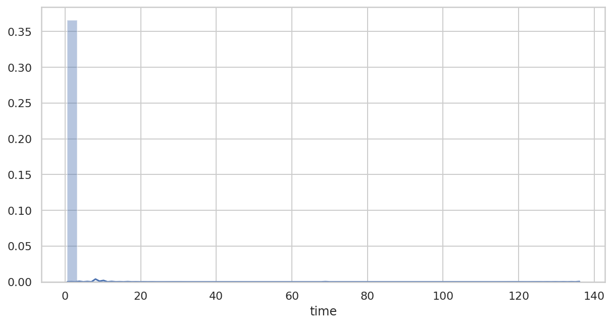
以上两个图基本与积分正常时次的图形一致，看不出积分时间异常的原因。

分析

对数据进行简单的分析。

时间分析

积分总时间，单位为分钟

edf["time"].sum()/60

92.71555

积分时间明显延长。

积分耗时大于 1s 步骤的总时间，单位为分钟

edf["time"][edf["time"]>1].sum()/60

92.69992166666667

可见，绝大部分步骤的耗时都大于 1s。

积分耗时大于 2s 步骤的总时间，单位为分钟

edf["time"][edf["time"]>2].sum()/60

10.903523333333336

虽然耗时大于 2s 的步骤占 10 分钟，但明显 1s 到 2s 之间的步骤耗时更多，也是积分时间延长的主要因素。

直方图

上面的直方图细节不够明显，我们再一次绘制直方图，不过只选择耗时小于 2s 的步骤。

正常数据：

fig, ax = plt.subplots(figsize=(10, 5))
sns.distplot(
    df["time"][df["time"] < 2],
    ax=ax
)

异常数据：

fig, ax = plt.subplots(figsize=(10, 5))
sns.distplot(
    edf["time"][edf["time"] < 2],
    ax=ax
)

从这两张图中可以看到，第一个数据单步积分时间大都在 0.6-0.8s 之间，而第二个数据在 1.0-1.2s 之间。

虽然相差不大，但对于 4000-5000 步来讲，累积效应还是很明显。

折线图

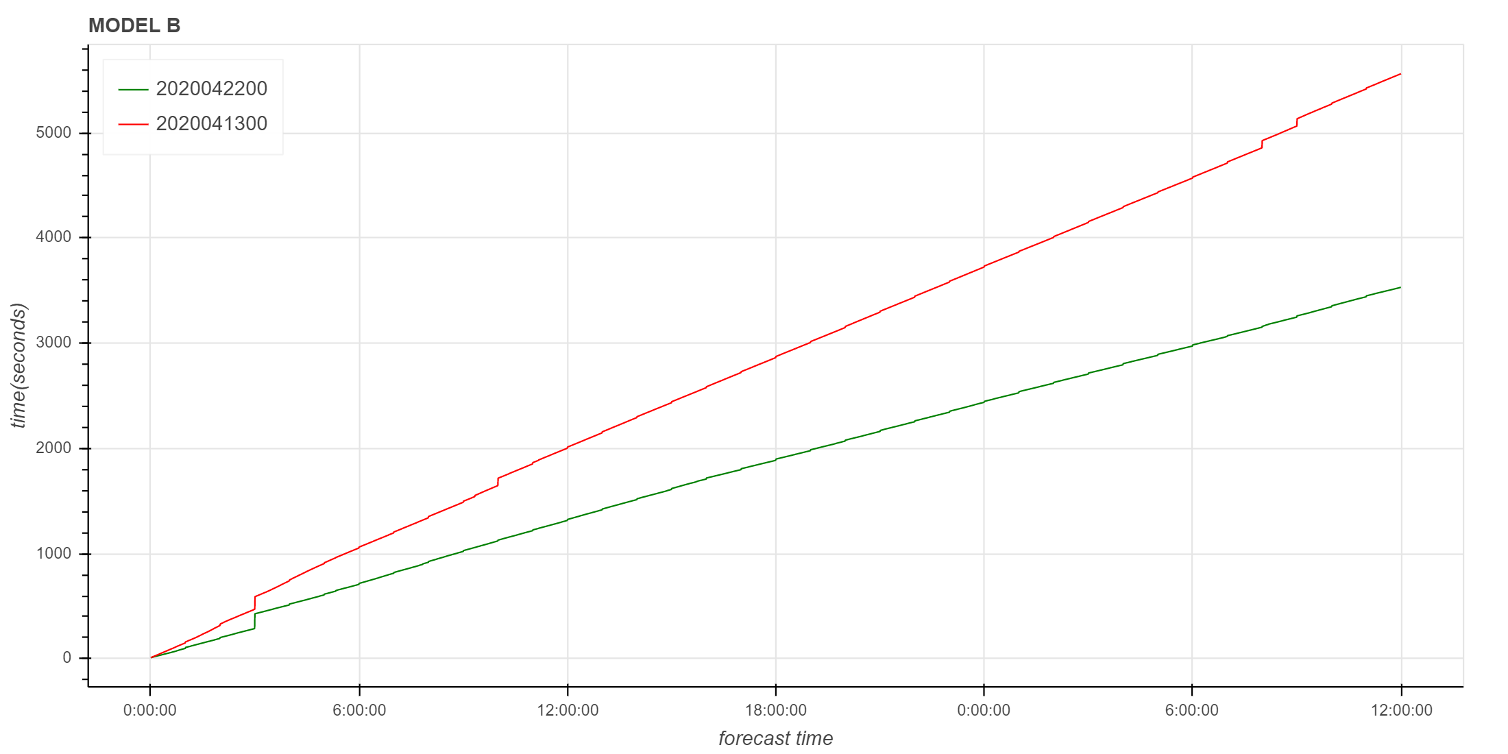
使用 Bokeh 绘制两个时次的累计时间图

from bokeh.io import output_notebook, show
from bokeh.plotting import figure
output_notebook()

from bokeh.models import ColumnDataSource, DatetimeTickFormatter

source = ColumnDataSource(df)
esource = ColumnDataSource(edf)

formatter = DatetimeTickFormatter(
    minsec=['%H:%M:%S'],
    minutes=['%H:%M:%S'],
    hourmin=['%H:%M:%S'],
    hours=['%H:%M:%S'],
    days=['%H:%M:%S'],
)


p = figure(
    plot_height=500,
    plot_width=1000,
    title="MODEL B",
    x_axis_type="datetime",
)

p.line(
    x="forecast_time",
    y="ctime",
    source=source,
    legend_label="2020042200",
    line_color="green",
)

p.line(
    x="forecast_time",
    y="ctime",
    source=esource,
    legend_label="2020041300",
    line_color="red",
)

p.legend.location = "top_left"
p.xaxis.axis_label = "forecast time"
p.xaxis.formatter = formatter
p.yaxis.axis_label = "time(seconds)"

show(p)

进一步对比

构造批量获取数据的函数

def get_cum_time(start_time_list):
    data = dict()
    for start_time in start_time_list:
        file_path = find_local_file(
            "grapes_meso_3km/log/fcst_ecf_out",
            start_time=start_time,
        )
        df = get_step_time_from_file(file_path)
        df["ctime"] = df["time"].cumsum()
        df["forecast_time"] = df["valid_time"] - start_time
        df["ctime"] = df["time"].cumsum()
        data[start_time] = df
    return data

获取 4 月 10 日至 4 月 30 日之间的数据，并打印积分总耗时。

data = get_cum_time(pd.date_range("2020-04-10", "2020-04-30", freq="D"))
for (key, df) in data.items():
    print(f"{key.strftime('%Y-%m-%d')} {df['time'].sum()/60:.2f}")

2020-04-10 58.08
2020-04-11 57.16
2020-04-12 56.84
2020-04-13 92.72
2020-04-14 58.39
2020-04-15 56.97
2020-04-16 57.08
2020-04-17 75.25
2020-04-18 59.96
2020-04-19 61.97
2020-04-20 63.41
2020-04-21 61.34
2020-04-22 59.57
2020-04-23 56.34
2020-04-24 57.78
2020-04-25 58.39
2020-04-26 55.69
2020-04-27 56.63
2020-04-28 56.94
2020-04-29 94.79
2020-04-30 58.87

有两天的耗时明显异常：2020-04-13 和 2020-04-29。 2020-04-17 的时间也应该不属于正常范围。

使用 Bokeh 绘制以上数据的折线图。

from bokeh.io import output_notebook, show
from bokeh.plotting import figure
from bokeh.palettes import viridis
from bokeh.models import Legend, LegendItem, PrintfTickFormatter, ColumnDataSource
from bokeh.models.formatters import DatetimeTickFormatter

output_notebook()

colormap = viridis(len(data))

p = figure(
    plot_height=500,
    plot_width=1000,
    title="MODEL B",
)

i = 0
items = []
for (key, df) in data.items():
    df["forecast_hour"] = df["forecast_time"] / pd.Timedelta(hours=1)
    source = ColumnDataSource(df)
    l = p.line(
        x="forecast_hour",
        y="ctime",
        source=source,
        color=colormap[i],
    )
    items.append(
        LegendItem(
            label=key.strftime("%Y-%m-%d"), 
            renderers=[l],
        )
    )
    i += 1
    
p.xaxis.axis_label = "forecast time"
p.yaxis.axis_label = "time(seconds)"

p.xaxis.bounds = (0, 36)
p.xaxis.formatter = PrintfTickFormatter(format="%dh")

legend = Legend(
    items=items, 
    location="center",
)

p.add_layout(legend, 'right')
    
show(p)