NWPC笔记：分析模式积分时长 - 线性回归

May 10, 2020 (最后修改: August 22, 2021)

meteorology/devops

上一篇文章《NWPC笔记：对比模式积分时长 - 恒定步长》中提到模式积分单步耗时累计时间在正常情况和异常情况下有不同的斜率。

本文介绍使用线性回归拟合模式积分单步耗时，并对比两种情况下线性拟合的效果。

声明：本文仅代表作者个人观点，所用数据无法代表真实情况，严禁转载。关于模式系统的相关信息，请以官方发布的信息及经过同行评议的论文为准。

获取数据

使用《NWPC笔记：对比模式积分时长 - 恒定步长》中提到的 2020 年 4 月 13 日（异常情况）和 2020 年 5 月 5 日（正常情况）两个数据。具体获取方法请查看该文章，不再详细介绍。

下面首先以 2020 年 5 月 5 日的数据为例说明如何进行线性拟合。

假设数据已被加载到 df 中。

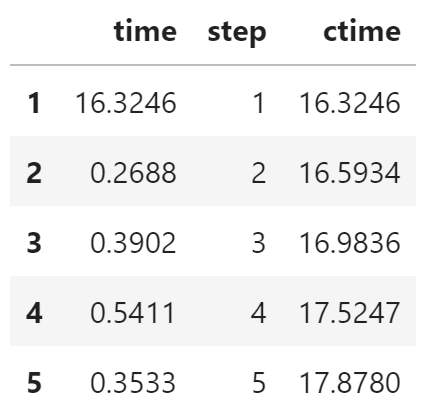
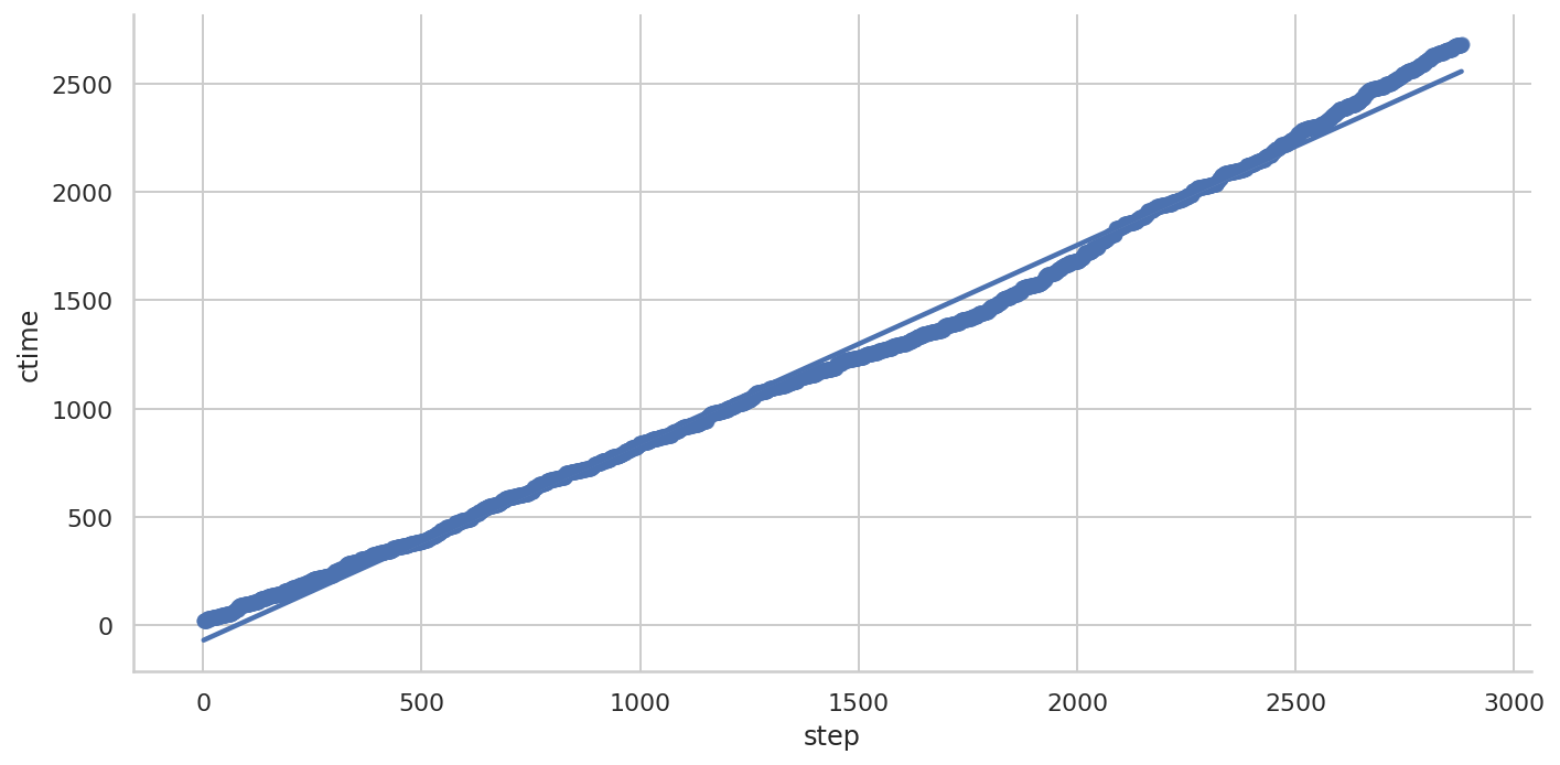
使用 Seaborn 绘制线性拟合曲线

Seaborn 内置了线性拟合功能。

import seaborn as sns
sns.set(style="whitegrid")

sns.lmplot(
    x="step", 
    y="ctime", 
    data=df,
    height=5,
    aspect=2,
)

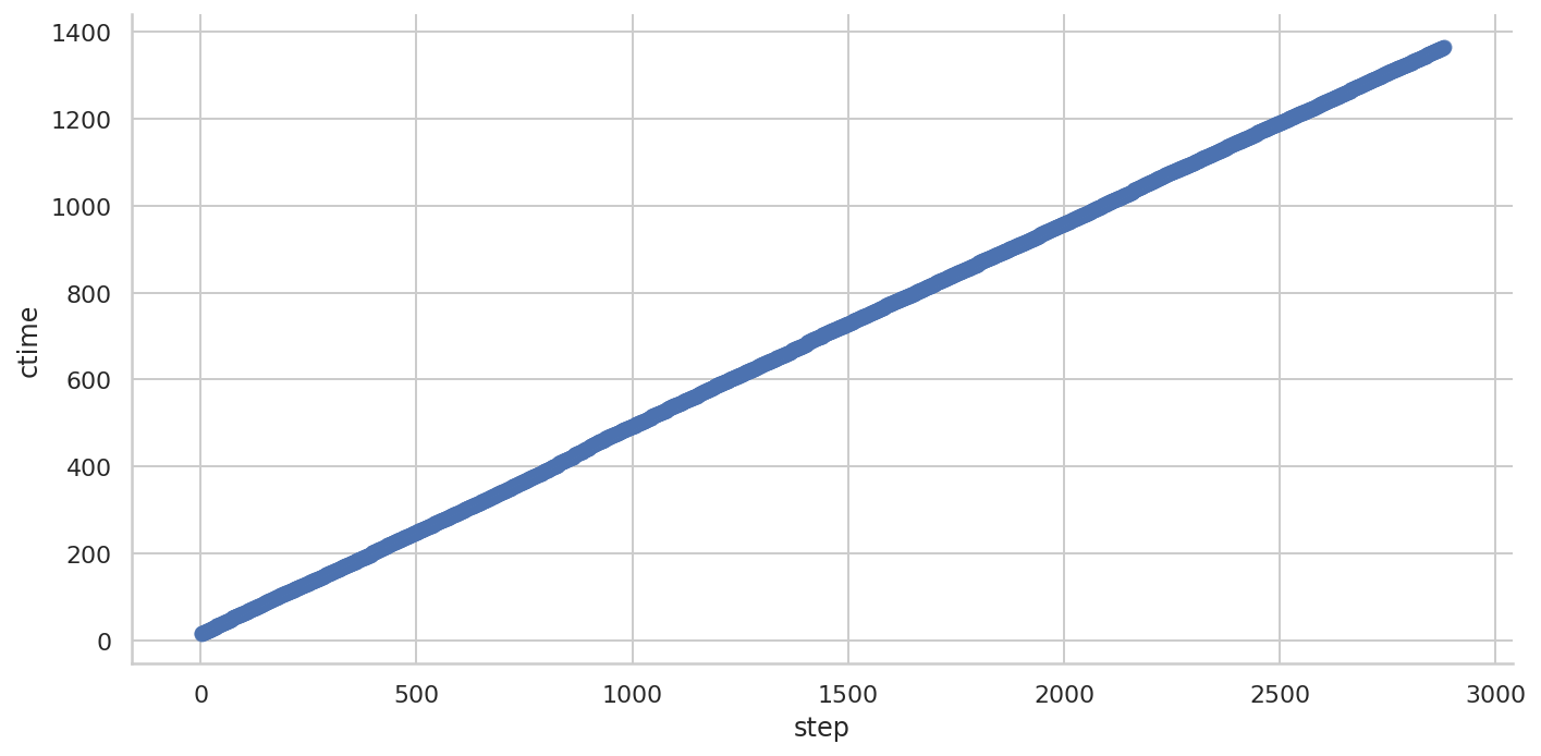
点数量太多，导致拟合直线和数据点混在一块，也说明了正常情况下的数据有很好的线性关系。

使用 scikit-learn 计算线性回归

使用 scikit-learn 提供的线性回归算法 LinearRegression 计算线性拟合。

from sklearn import linear_model

将积分步数处理成 scikit-learn 需要的二维变量。

X = df["step"].values.reshape(-1, 1)
y = df["ctime"]

使用所有的数据训练线性回归模型（不是最好的方式）

reg = linear_model.LinearRegression()
reg.fit(X, y)

LinearRegression(copy_X=True, fit_intercept=True, n_jobs=None, normalize=False)

查看拟合直线的斜率和截距

reg.coef_, reg.intercept_

(array([0.4696361]), 18.332078275562708)

查看拟合的评分

reg.score(X, y)

0.9998938918125222

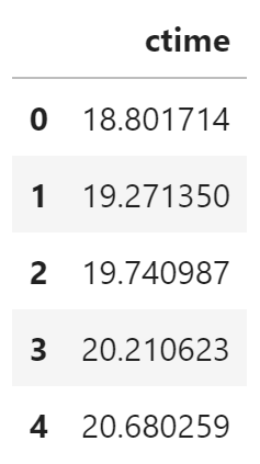
使用训练的模型计算累计时间

predict_df = pd.DataFrame(
    {
        "ctime": reg.predict(
            df["step"].values.reshape(-1, 1)
        )
    }
)
predict_df.head()

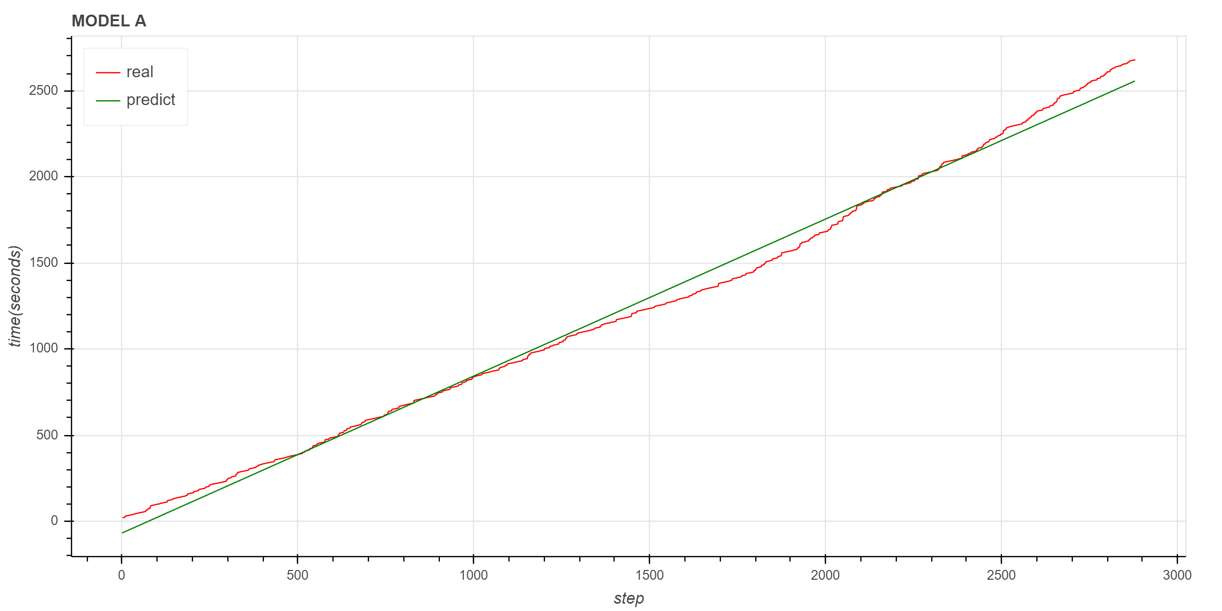
下面使用 Bokeh 绘制原始数据和预测数据的折线图。

from bokeh.io import output_notebook, show
from bokeh.plotting import figure
from bokeh.models import ColumnDataSource
output_notebook()

source = ColumnDataSource(df)
predict_source = ColumnDataSource(predict_df)

p = figure(
    plot_height=500,
    plot_width=1000,
    title="MODEL A",
)
p.line(
    x="step",
    y="ctime",
    source=source,
    color="red",
    legend_label="real"
)

p.line(
    x="index",
    y="ctime",
    source=predict_source,
    color="green",
    legend_label="predict",
)

p.legend.location = "top_left"
p.xaxis.axis_label = "step"
p.yaxis.axis_label = "time(seconds)"

show(p)

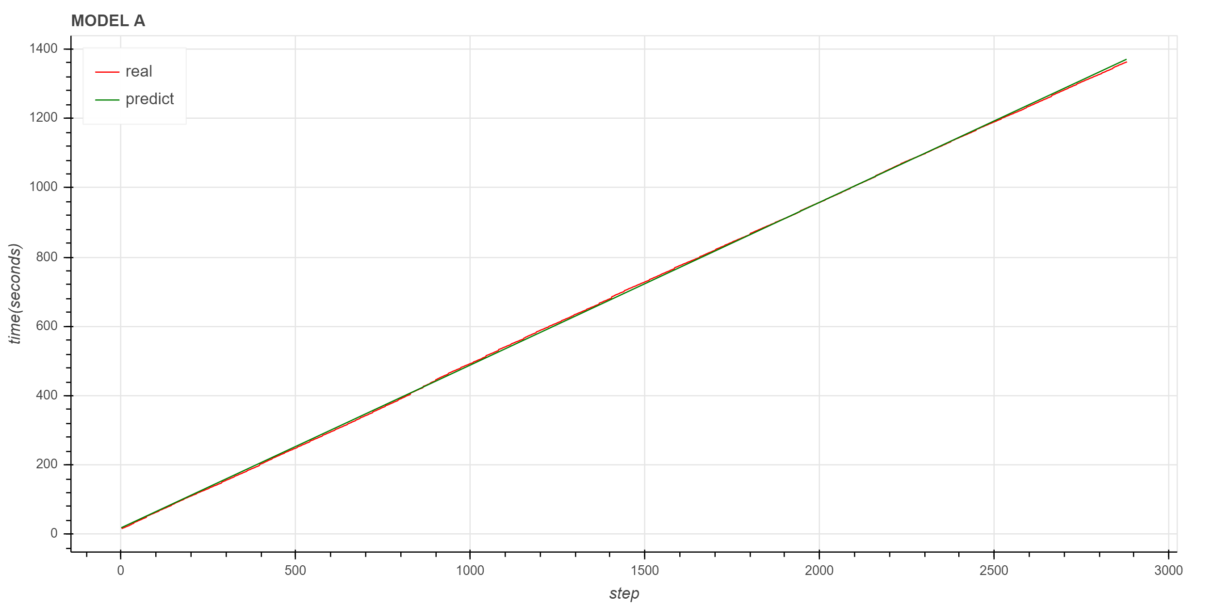
图中红色是实际曲线，绿色是拟合的直线，拟合直线很好地描述了实际数据的变化趋势。

异常情况

下面让我们再看一下异常情况下线性拟合的效果。

Seaborn

Seaborn 的线性拟合

可以看到拟合的曲线与实际数据有较大的差异。

Scikit-learn

使用 scikit-learn 训练线性回归模型

斜率和截距

(array([0.91139774]), -69.14379092405215)

拟合效果评分

0.993858593974111

实际数据与拟合数据对比

同样可以看到，拟合直线对原始数据的描述不太理想。笔者后续会继续寻找适合原始数据的拟合方法。

进一步评估

下面查看 2020 年 4 月 10 日到 4 月 30 日的拟合结果。

获取数据

def get_cum_time(start_time_list):
    data = dict()
    for start_time in start_time_list:
        file_path = find_local_file(
            "grapes_gfs_gmf/log/fcst_long_std_out",
            start_time=start_time,
        )
        df = get_step_time_from_file(file_path)
        df["ctime"] = df["time"].cumsum()
        data[start_time] = df["ctime"]
    df = pd.DataFrame(
        data, 
        index=df.index
    )
    return df

df = get_cum_time(pd.date_range("2020-04-10", "2020-04-30", freq="D"))
df.iloc[-1] / 60

2020-04-10    23.170123
2020-04-11    23.935507
2020-04-12    22.960625
2020-04-13    44.652387
2020-04-14    23.098123
2020-04-15    22.748205
2020-04-16    22.902938
2020-04-17    23.128332
2020-04-18    23.376948
2020-04-19    23.527448
2020-04-20    22.829743
2020-04-21    32.210792
2020-04-22    29.892152
2020-04-23    23.042733
2020-04-24    22.938663
2020-04-25    22.867722
2020-04-26    22.937087
2020-04-27    31.016060
2020-04-28    32.708422
2020-04-29    31.268345
2020-04-30    22.859272
Name: 2880, dtype: float64

计算模型并输出拟合结果

end_times = []
days = 10
sample_number = 12 * 24 * days
test_number = 2880 - sample_number
if test_number == 0:
    test_number = 0
for a in df:
    X = df[a].index.values.reshape(-1, 1)
    y = df[a]
    reg = linear_model.LinearRegression()
    reg.fit(X[:sample_number], y[:sample_number])
    end_time = reg.predict(np.reshape(2880, (-1, 1)))[0]/60
    print(a, reg.coef_, df[a].iloc[-1]/60, end_time)
    end_times.append(end_time)

2020-04-10 00:00:00 [0.48077122] 23.170123333333414 23.363564776374954
2020-04-11 00:00:00 [0.49622826] 23.935506666666722 24.264343912572585
2020-04-12 00:00:00 [0.47620212] 22.960624999999986 23.239307100219186
2020-04-13 00:00:00 [0.91139774] 44.652386666666686 42.594695147925194
2020-04-14 00:00:00 [0.47821313] 23.098123333333294 23.284127955883513
2020-04-15 00:00:00 [0.46963779] 22.74820500000002 22.816283634990842
2020-04-16 00:00:00 [0.47342688] 22.902938333333324 23.089884599234118
2020-04-17 00:00:00 [0.47983486] 23.128331666666618 23.26621174881766
2020-04-18 00:00:00 [0.48406351] 23.376948333333242 23.53075427557699
2020-04-19 00:00:00 [0.48439856] 23.527448333333282 23.654108120745143
2020-04-20 00:00:00 [0.46991823] 22.829743333333344 22.978980555945245
2020-04-21 00:00:00 [0.66293275] 32.21079166666669 32.662045968569636
2020-04-22 00:00:00 [0.61786773] 29.892151666666646 30.061560073844657
2020-04-23 00:00:00 [0.47533177] 23.042733333333306 23.159868435623824
2020-04-24 00:00:00 [0.47643454] 22.93866333333335 23.169338820445194
2020-04-25 00:00:00 [0.47379122] 22.867721666666665 23.12351359681649
2020-04-26 00:00:00 [0.47331713] 22.937086666666758 23.15515623762936
2020-04-27 00:00:00 [0.64281024] 31.016059999999978 31.16133771762634
2020-04-28 00:00:00 [0.67747214] 32.70842166666656 32.83951449666227
2020-04-29 00:00:00 [0.6435027] 31.268345000000018 31.489873762310086
2020-04-30 00:00:00 [0.47057938] 22.859271666666668 22.94356791260509

上面输出中第二列是斜率，第三列是实际时间，第四列是拟合时间。可以看到，积分耗时大的时次，拟合的斜率也比较大。

计算最后一步拟合结果与实际数据的偏差

end_times - df.iloc[-1]/60

2020-04-10   -0.236164
2020-04-11   -0.267531
2020-04-12    0.134403
2020-04-13   -8.333957
2020-04-14   -0.130312
2020-04-15   -0.624128
2020-04-16    0.451455
2020-04-17   -0.561062
2020-04-18    0.003283
2020-04-19    0.651331
2020-04-20    0.727592
2020-04-21   -0.683699
2020-04-22    0.113455
2020-04-23    0.139197
2020-04-24   -0.264757
2020-04-25    0.108965
2020-04-26    0.019950
2020-04-27    0.197263
2020-04-28    0.157849
2020-04-29    0.849784
2020-04-30    0.670015
Name: 2880, dtype: float64

可以看到，除了 4 月 13 日的偏差比较大外，其余偏差均在 1 分钟内。而 4 月 13 日的偏差虽然有 8 分钟，但实际数据减去 8 分钟依然处在异常范围内。

使用全量数据训练模型没有太大意义，我们更关心是否能在模式运行阶段就预测出模式积分有异常，这就需要使用前面积分步骤的耗时数据来预测积分的总体趋势。下一篇文章将尝试讨论使用部分数据预测的可行性。

参考

https://github.com/nwp-oper/nwpc-log-tool

《NWPC笔记：对比模式积分时长 - 恒定步长》