NWPC笔记:对比模式积分时长 - 恒定步长
上一篇文章《NWPC笔记:获取模式积分时长 - 恒定步长》介绍如何从模式输出日志获取模式积分每步的时长,并绘制一些统计图形。选用的是模式积分耗时处于正常范围内的时次。 但从文章《统计数值天气预报模式积分运行时间》中可以看到,个别情况下模式积分时长会显著增加。
本文使用《NWPC笔记:获取模式积分时长 - 恒定步长》中的方法,对比 GRAPES GFS 模式积分耗时正常和异常情况下每步积分的时长变化。
声明:本文仅代表作者个人观点,所用数据无法代表真实情况,严禁转载。关于模式系统的相关信息,请以官方发布的信息及经过同行评议的论文为准。
获取数据
以下假设已按照前一篇文章中的方法,将积分时间正常的 2020050500 时次的数据保存到 df 中。
加载积分时间超时的 2020041300 时次的数据。
file_path = find_local_file(
"grapes_gfs_gmf/log/fcst_long_std_out",
start_time="2020041300",
)
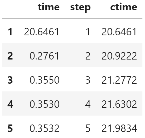
edf = get_step_time_from_file(file_path)
edf["step"] = edf.index
edf["ctime"] = edf["time"].cumsum()
edf.head()
绘制统计图形
与前一篇文章一样,使用 Seaborn 绘制统计图形
import seaborn as sns
sns.set(style="whitegrid")
折线图
fig, ax = plt.subplots(figsize=(20, 5))
sns.lineplot(
    x="step",
    y="time",
    data=edf[1:],
    ax=ax
)
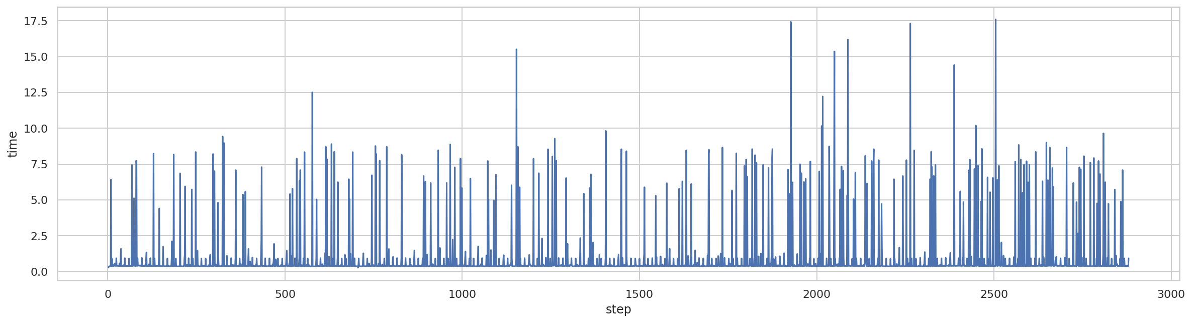
可以看到,4 月 13 日 00 时次的积分单步耗时明显比 5 月 5 日 00 时次多,甚至出现单步耗时 17 秒的情况。
直方图
fig, ax = plt.subplots(figsize=(20, 5))
sns.distplot(
    edf["time"][1:],
    ax=ax
)
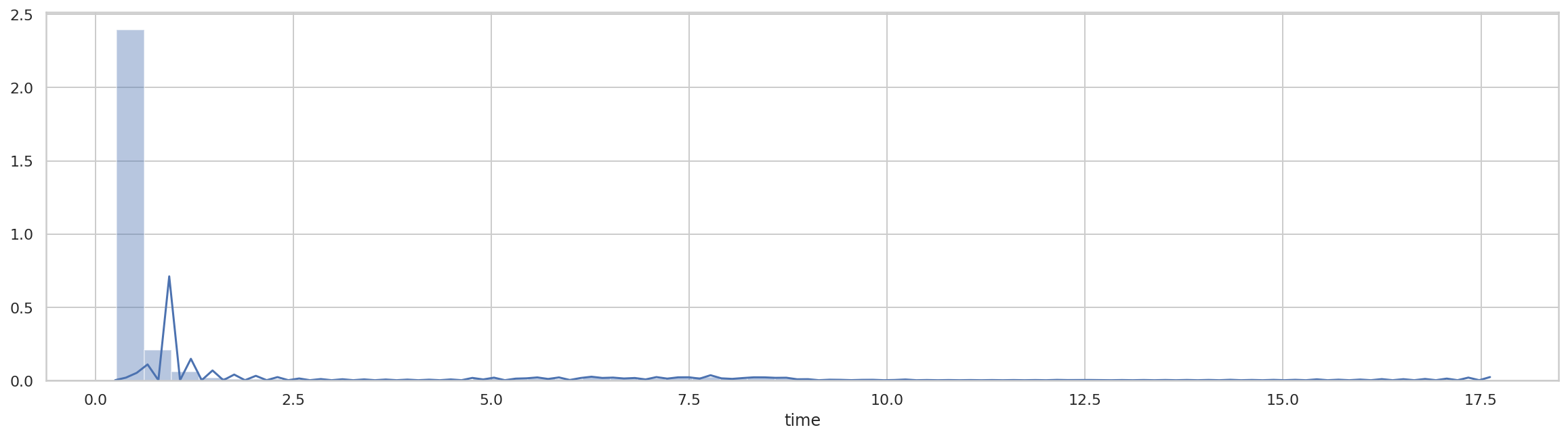
同样可以看到,虽然大部分步骤依然耗时在 0.5 秒以内,但步骤耗时分布区间明显增大。
简单分析
所有步骤耗时,单位为分钟。
edf["time"].sum()/60
44.65238666666667
耗时几乎是 5 月 5 日 00 时次的 2 倍。
耗时大于 1 秒的步骤的累计时间,单位为分钟。
edf["time"][edf["time"]>1].sum()/60
25.928708333333336
大于 1 秒步骤的总时间几乎占到一半,模式积分时间延长主要受这些步骤的影响。
绘制累计时间折线图
fig, ax = plt.subplots(figsize=(10, 5))
edf["ctime"].plot(
    ax=ax
)
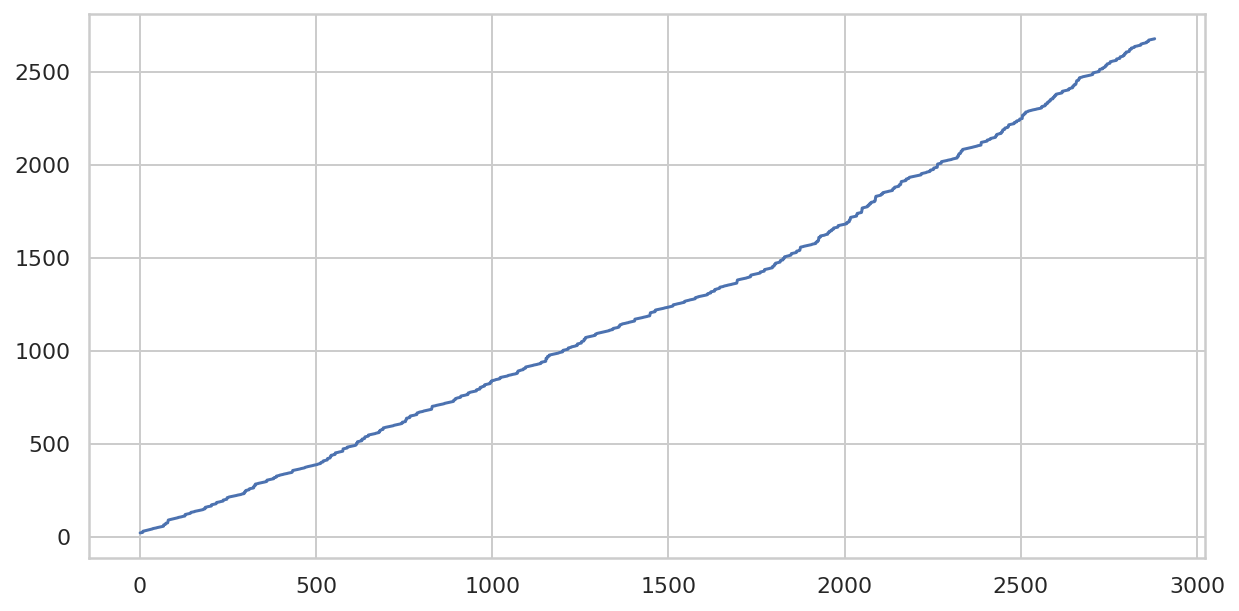
折线图看起来不像是一条直线。
对比显示
使用 Bokeh 同时绘制前一篇文章的正常情况数据和本文新获取的异常情况数据。
加载需要的模块
from bokeh.io import output_notebook, show
from bokeh.plotting import figure
from bokeh.models import ColumnDataSource
output_notebook()
创建 Bokeh 需要的数据
normal_source = ColumnDataSource(df)
late_source = ColumnDataSource(edf)
绘制图形
p = figure(
    plot_height=500,
    plot_width=1000,
    title="MODEL A",
)
p.line(
    x="step",
    y="ctime",
    source=normal_source,
    color="green",
    legend_label="2020050500"
)
p.line(
    x="step",
    y="ctime",
    source=late_source,
    color="red",
    legend_label="2020041300"
)
p.legend.location = "top_left"
p.xaxis.axis_label = "step"
p.yaxis.axis_label = "time(seconds)"

show(p)
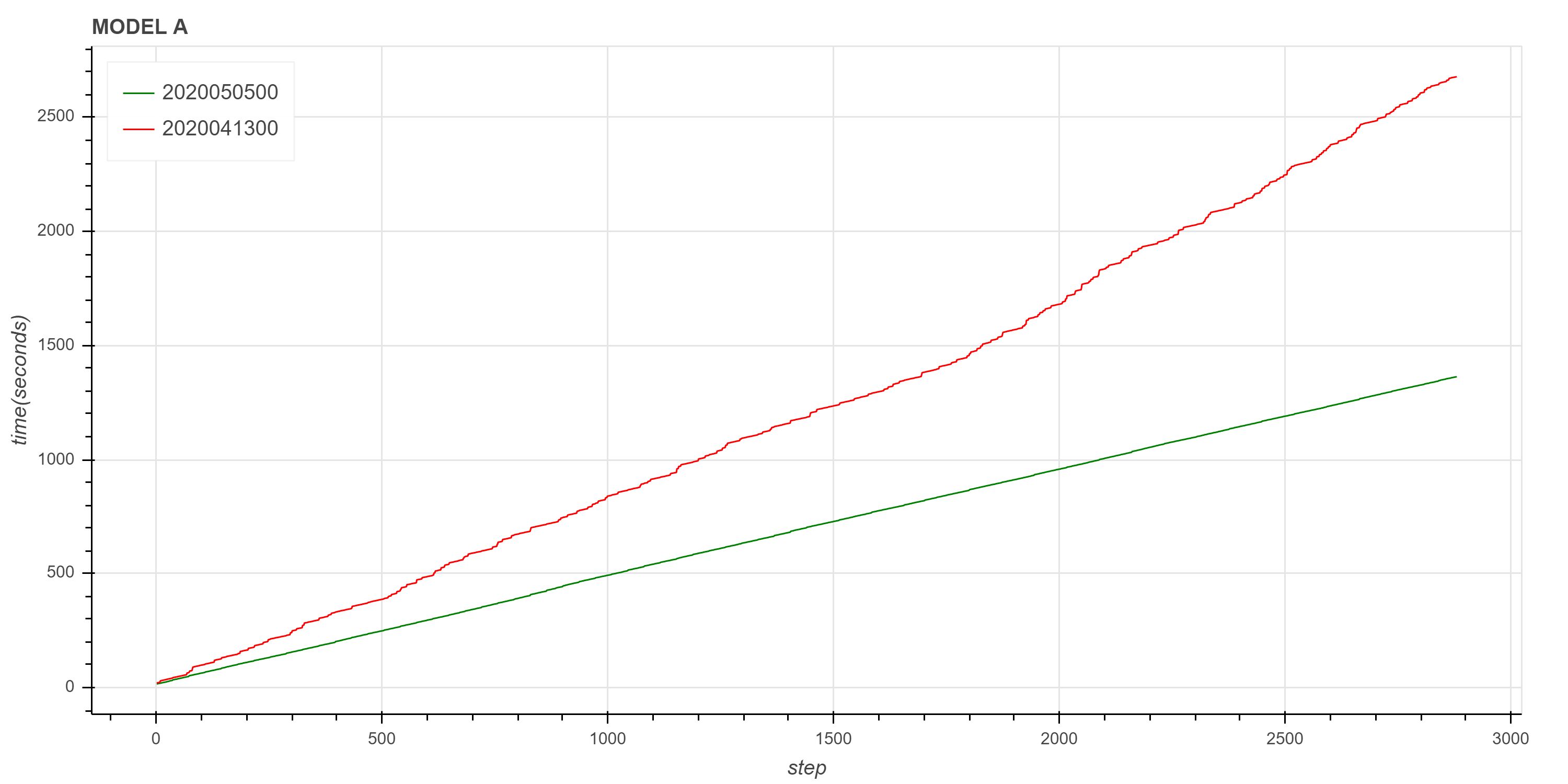
可以看到,正常情况下积分累计时间近似于一条直线,但 4 月 13 日 00 时次的异常情况则没有这样的特性,虽然也可以看成是保持线性趋势的。
进一步对比
为了进一步验证正常和异常情况下积分累计时间的趋势,下面绘制从 4 月 20 日到 4 月 30 日共计 11 天的积分步骤累计时间图。
首先创建批量获取数据的函数。
def get_cum_time(start_time_list):
    data = dict()
    for start_time in start_time_list:
        file_path = find_local_file(
            "grapes_gfs_gmf/log/fcst_long_std_out",
            start_time=start_time,
        )
        df = get_step_time_from_file(file_path)
        df["ctime"] = df["time"].cumsum()
        data[start_time] = df["ctime"]
    df = pd.DataFrame(
        data,
        index=df.index
    )
    return df
获取数据
total_df = get_cum_time(
    pd.date_range(
        "2020-04-20",
        "2020-04-30",
        freq="D"
    )
)
total_df.head()
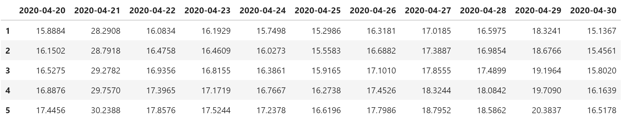
查看每个时次的积分累计时间
total_df.iloc[-1]/60
2020-04-20    22.829743
2020-04-21    32.210792
2020-04-22    29.892152
2020-04-23    23.042733
2020-04-24    22.938663
2020-04-25    22.867722
2020-04-26    22.937087
2020-04-27    31.016060
2020-04-28    32.708422
2020-04-29    31.268345
2020-04-30    22.859272
Name: 2880, dtype: float64
上述数据中,有 5 个时次的积分时间明显延长:
- 2020-04-21:32.210792
- 2020-04-22:29.892152
- 2020-04-27:31.016060
- 2020-04-28:32.708422
- 2020-04-29:31.268345
使用 Bokeh 画图
from bokeh.palettes import viridis

colormap = viridis(len(source_df.columns))
source = ColumnDataSource(source_df)

p = figure(
    plot_height=500,
    plot_width=1000,
    title="MODEL A",
)

i = 0
for col in source_df.columns:
    p.line(
        x="index",
        y=col,
        source=source,
        color=colormap[i],
        legend_label=col
    )
    i += 1

p.legend.location="top_left"
p.xaxis.axis_label = "step"
p.yaxis.axis_label = "time(seconds)"

show(p)
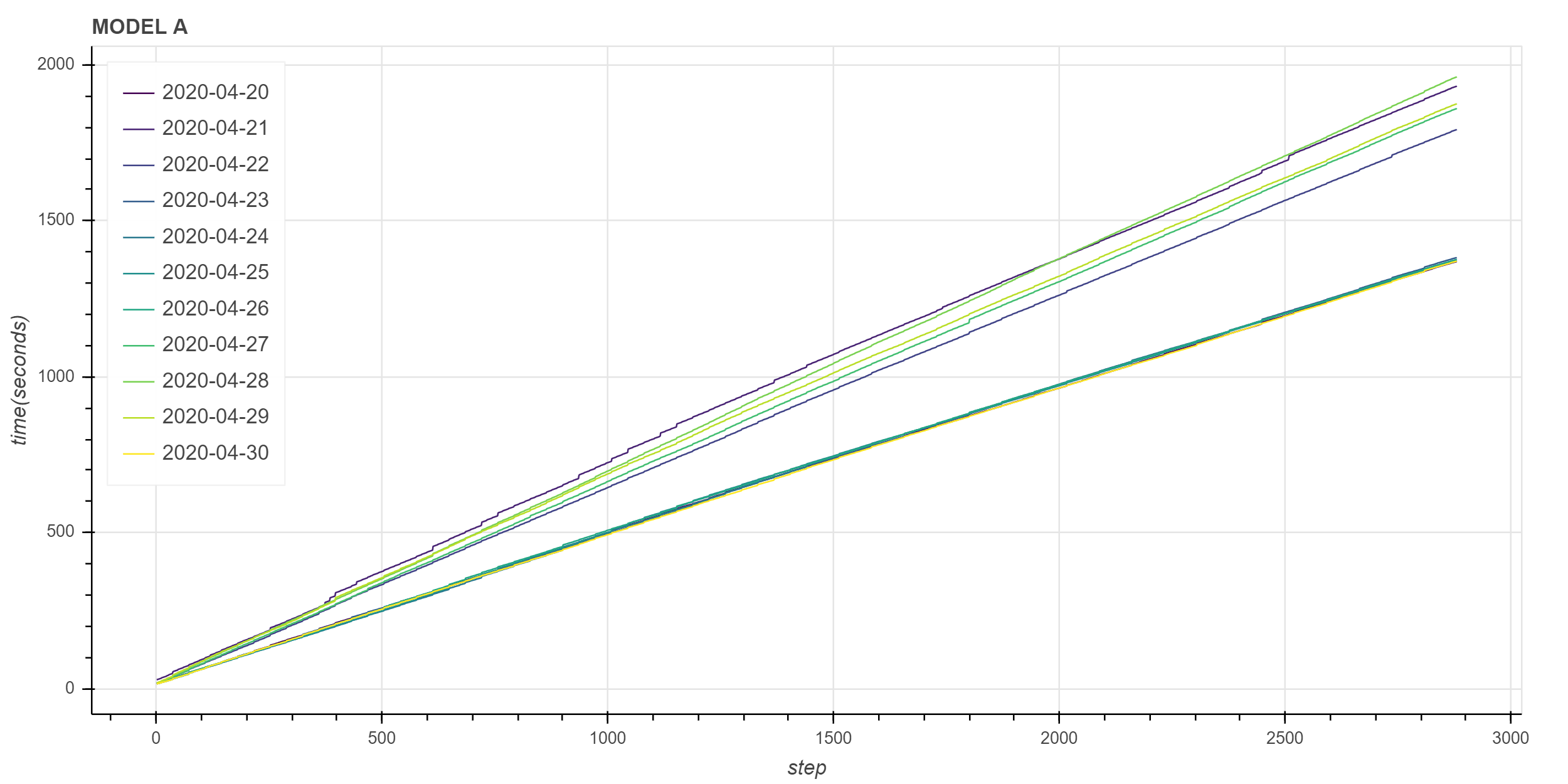
可以看到,有 5 条线段的斜率明显比其它线段大,而其它线段的斜率基本一致。 这说明积分时间与累计时间折线图的斜率有一定的关系。
下一篇文章将会介绍如何计算积分累计时间的斜率,即积分累计时间与积分步数的线性关系。
