统计数值预报产品生成时间:重采样
目录
之前的文章《统计数值天气预报模式产品生成的典型时间》中介绍根据GRIB2文件创建时间统计产品生成的典型时间,并在《统计数值预报产品生成时间:单个时效重采样》中介绍使用重采样技术统计单个时效的生成时间。
本文基于这两篇文章,介绍如何使用自助法统计 所有 时效产品的生成时间。
声明:本文仅代表作者个人观点,所用数据无法代表真实情况,严禁转载。关于模式系统的相关信息,请以官方发布的信息及经过同行评议的论文为准。
数据
载入需要使用的库
from pathlib import Path

import pandas as pd
import numpy as np
import matplotlib.pyplot as plt

from nwpc_data.data_finder import find_local_file
构造一个函数,批量获取文件创建时间
def calculate_time(
    data_type,
    date_range,
    forecast_hours,
):
    b = []
    for forecast_hour in forecast_hours:
        file_list=[
            find_local_file(
                data_type,
                start_time=t,
                forecast_time=forecast_hour
            )
            for t
            in date_range
        ]
        ts = [pd.to_datetime(Path(f).stat().st_mtime_ns) - pd.to_datetime(d.date())  for f, d in zip(file_list, date_range) ]
        s = pd.Series(ts, index=date_range)
        s.name = int(forecast_hour.seconds/3600) + forecast_hour.days * 24
        b.append(s)
    df = pd.DataFrame(b)
    df = df.T
    return df
构造起报时次列表
date_range = pd.date_range(
    "2020-03-01 00:00:00",
    "2020-04-29 00:00:00",
    freq="D"
)
构造时效列表
forecast_hours = [
    pd.Timedelta(hours=h)
    for h in
    np.append(
        np.arange(0, 121, 3),
        np.arange(126, 241, 6)
    )
]
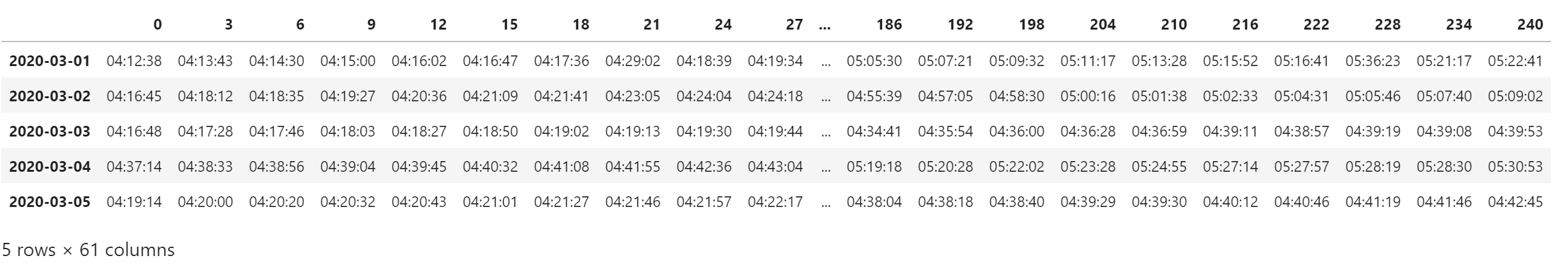
计算时间段内所有时效文件的创建时间
df = calculate_time(
  "grapes_gfs_gmf/grib2/orig",
  date_range,
  forecast_hours
)
df.head()
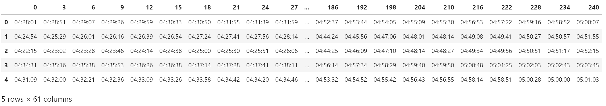
重采样
对数据进行重采样,每次选择 20 个样本,重复 10000 次。 计算每次采样的均值。
注意:本文采样单位是 df 中的一行,即同一个时次各个时效的生成时间。
count = 10000
means = []
for i in range(0, count):
    sampled_data = df.sample(n=20, replace=True)
    means.append(sampled_data.mean())

bdf = pd.DataFrame(means).applymap(lambda x: x.ceil("s"))
bdf.head()
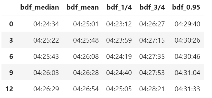
计算重采样数据的统计量
stat_df = pd.DataFrame(
    {
        "bdf_median": bdf.median(),
        "bdf_mean": bdf.mean(),
        "bdf_1/4": bdf.quantile(.25, numeric_only=False, interpolation="nearest"),
        "bdf_3/4": bdf.quantile(.75, numeric_only=False, interpolation="nearest"),
        "bdf_0.95": bdf.quantile(.95, numeric_only=False, interpolation="nearest"),
    }
)
stat_df = stat_df.applymap(lambda x: x.ceil("S"))
stat_df.head()
绘图
使用 Bokeh 绘制上面的统计量
from bokeh.io import output_notebook, show
from bokeh.plotting import figure
output_notebook()

from bokeh.models.formatters import DatetimeTickFormatter

data = stat_df
p = figure(
    plot_width=1000,
    plot_height=600,
    y_axis_type="datetime",
    title="MODEL A GRIB2 ORIG",
)

p.yaxis.formatter = DatetimeTickFormatter(
    minsec=['%H:%M:%S'],
    minutes=['%H:%M:%S'],
    hourmin=['%H:%M:%S'],
    hours=['%H:%M:%S']
)

p.line(
    data.index,
    data['bdf_mean'],
    line_color="SkyBlue",
    legend_label="bdf_mean",
)
p.line(
    data.index,
    data['bdf_1/4'],
    line_color="Pink",
    legend_label="bdf_1/4",
)
p.line(
    data.index,
    data['bdf_median'],
    line_color="green",
    legend_label="bdf_1/2",
)
p.line(
    data.index,
    data['bdf_3/4'],
    line_color="Purple",
    legend_label="bdf_3/4",
)
p.line(
    data.index,
    data['bdf_0.95'],
    line_color="Salmon",
    legend_label="bdf_0.95",
)

p.xaxis.axis_label = "forecast hour"
p.yaxis.axis_label = "clock"
p.legend.location = "top_left"

show(p)
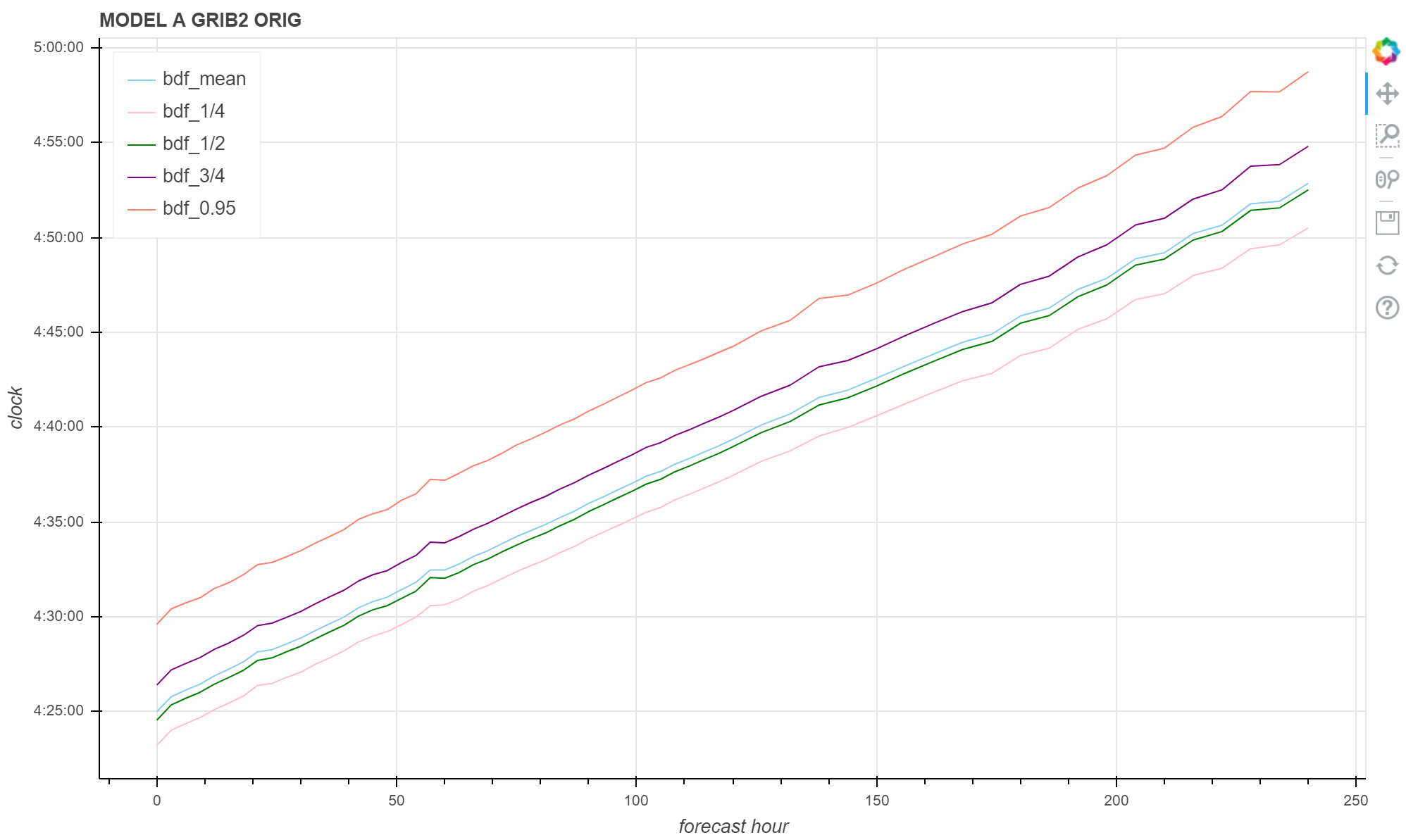
可以看到重采样后的数据无论是均值、中位数、四分位数还是 95% 分位点都保持基本相同的趋势。
数据分布
使用 Seaborn 绘制箱线图
import seaborn as sns
sns.set(style="whitegrid")
原始数据
ax = sns.catplot(
    data=df/pd.Timedelta(hours=1),
    orient="v",
    kind="box"
)
ax.fig.set_size_inches(25, 8)

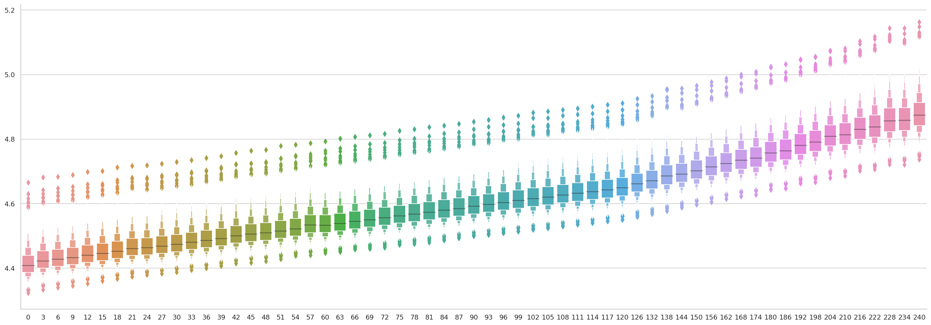
重采样后的数据
ax = sns.catplot(
    data=bdf/pd.Timedelta(hours=1),
    orient="v",
    kind="boxen"
)
ax.fig.set_size_inches(25, 8)
统计趋势
使用 Seaborn 绘制线性回归示意图。
单个时次
线性拟合单个时次,选择 6 个数据作为代表。
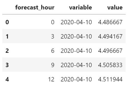
d = df.loc[pd.date_range("2020-04-10", "2020-04-15", freq="D")].T
d = d.apply(lambda x: x/pd.Timedelta(hours=1))
d["forecast_hour"] = d.index
d = d.melt(id_vars="forecast_hour")
d["variable"] = d["variable"].apply(lambda x: x.strftime("%Y-%m-%d"))
d.head()
为每个时次绘制线性回归
ax = sns.lmplot(
    x="forecast_hour",
    y="value",
    hue="variable",
    data=d,
)
ax.fig.set_size_inches(12, 8)
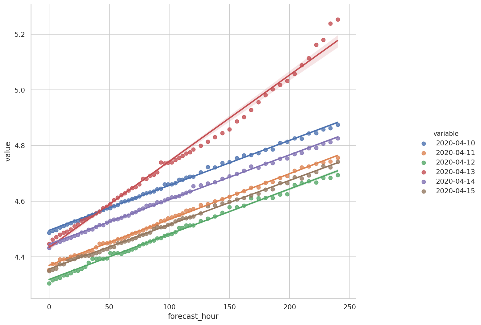
可以看到除了 4 月 13 日的红色线外,其余 5 条趋势线斜率基本一致。
从《统计数值预报产品生成时间:单个时效重采样》中的图形可以看到,4 月 13 日的 240 时效产品属于“延迟”类型,而其余 5 天均正常。
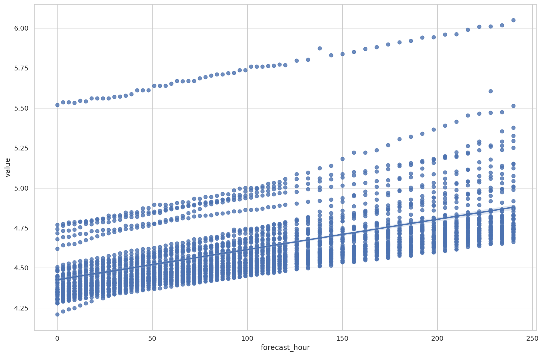
所有结果
线性拟合所有结果
df2 = df.T
df2["forecast_hour"] = df2.index
df3 = df2.melt(id_vars="forecast_hour")
df3["value"] = df3["value"]/pd.Timedelta(hours=1)

f, ax = plt.subplots(figsize=(15, 10))
sns.regplot(
    x="forecast_hour",
    y="value",
    data=df3,
    ax=ax,
)
线性拟合重采样的数据
df2 = bdf.T
df2["forecast_hour"] = df2.index
df3 = df2.melt(id_vars="forecast_hour")
df3["value"] = df3["value"]/pd.Timedelta(hours=1)

ax = sns.lmplot(
    x="forecast_hour",
    y="value",
    data=df3,
)
ax.fig.set_size_inches(15, 10)
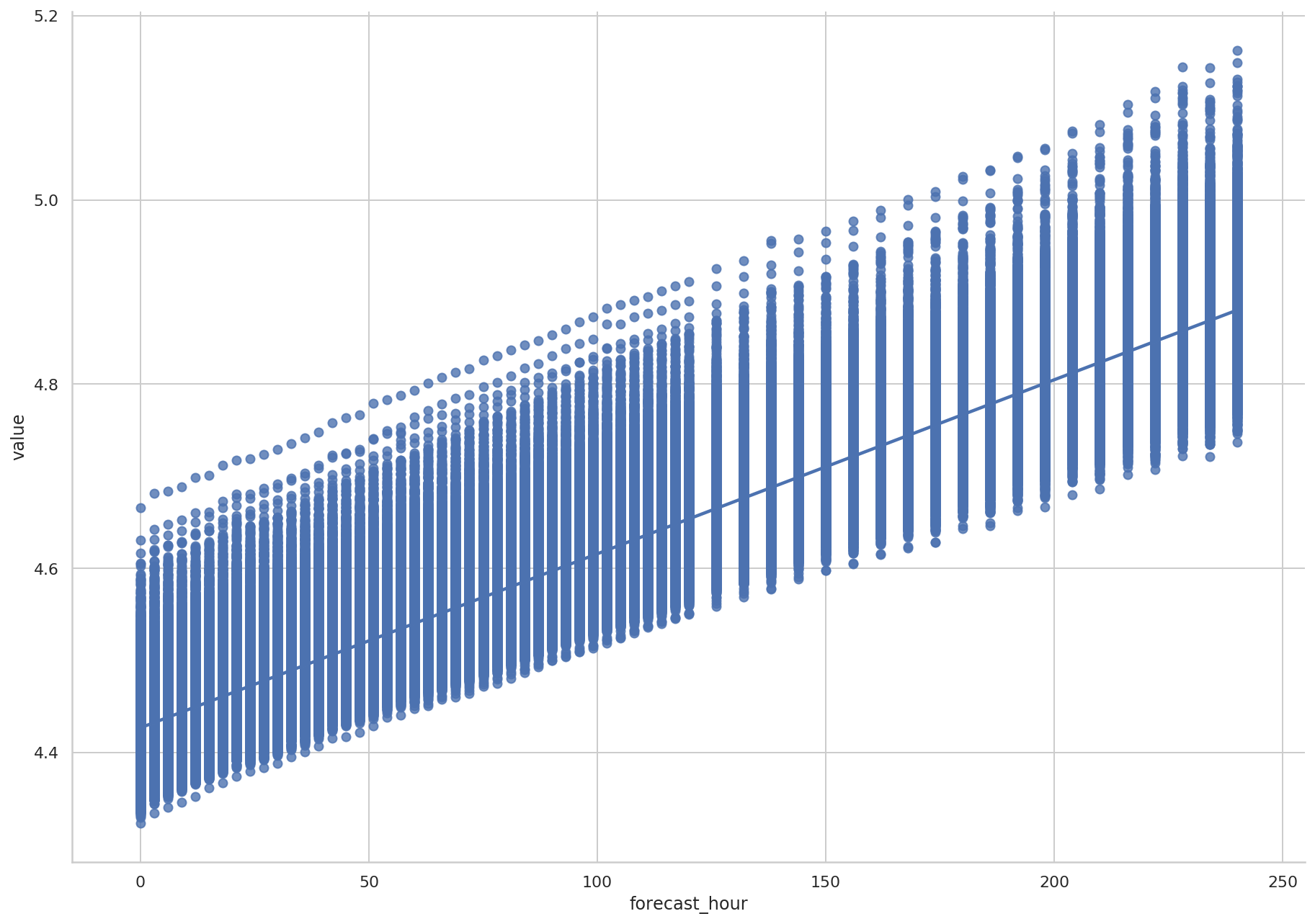
重采样后的数据趋势基本一致。
